Figure Gallery
66 figures from the thesis, filterable by chapter.
Ch. 2: Literature Survey
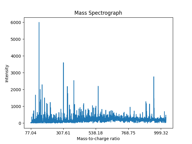
Figure 2.1: Mass Spectrograph: This is the artifact generated by Rapid Evaporative Ionization Mass Spectrometry (REIMS).
Figure 2.1: Mass Spectrograph: This is the artifact generated by Rapid Evaporative Ionization Mass Spectrometry (REIMS).
Ch. 2: Literature Survey
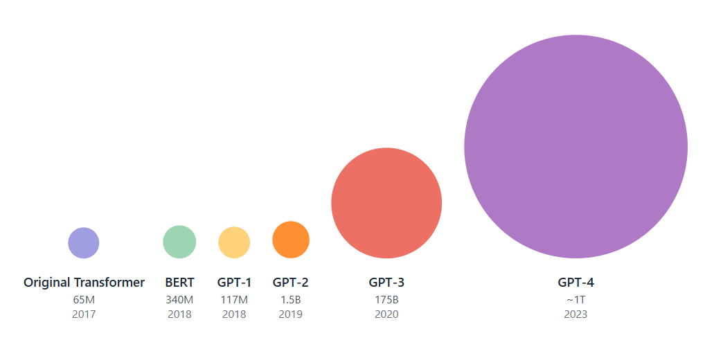
Figure 2.2: Illustrated here is a comparison of Transformer models, with each circle's size representing its approximate
Figure 2.2: Illustrated here is a comparison of Transformer models, with each circle's size representing its approximate
Ch. 2: Literature Survey
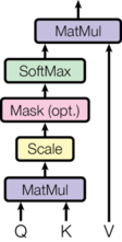
Figure 2.3: This figure illustrates the Scaled Dot-Product Attention mechanism , a core component of self-attention. It
Figure 2.3: This figure illustrates the Scaled Dot-Product Attention mechanism , a core component of self-attention. It
Ch. 2: Literature Survey
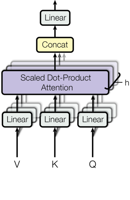
Figure 2.4: Multi-head attention enhances a model's ability to capture complex relationships by allowing it to jointly
Figure 2.4: Multi-head attention enhances a model's ability to capture complex relationships by allowing it to jointly
Ch. 3: Datasets and Processing
Figure 3.1: Mass Spectrograph: This is the artifact generated by Rapid Evaporative Ionization Mass Spectrometry (REIMS).
Figure 3.1: Mass Spectrograph: This is the artifact generated by Rapid Evaporative Ionization Mass Spectrometry (REIMS).
Ch. 3: Datasets and Processing
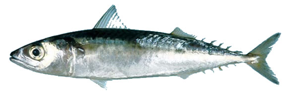
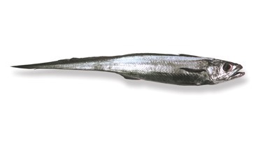
Mackerel — Figure 3.2: Mackerel (left), Hoki (right) fish species.
Mackerel — Figure 3.2: Mackerel (left), Hoki (right) fish species.
Ch. 3: Datasets and Processing
Hoki — Figure 3.2: Mackerel (left), Hoki (right) fish species.
Hoki — Figure 3.2: Mackerel (left), Hoki (right) fish species.
Ch. 3: Datasets and Processing
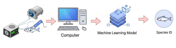
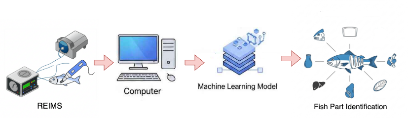
Figure 3.3: This diagram illustrates a machine learning model running on a computer to identify fish species. First, the
Figure 3.3: This diagram illustrates a machine learning model running on a computer to identify fish species. First, the
Ch. 3: Datasets and Processing
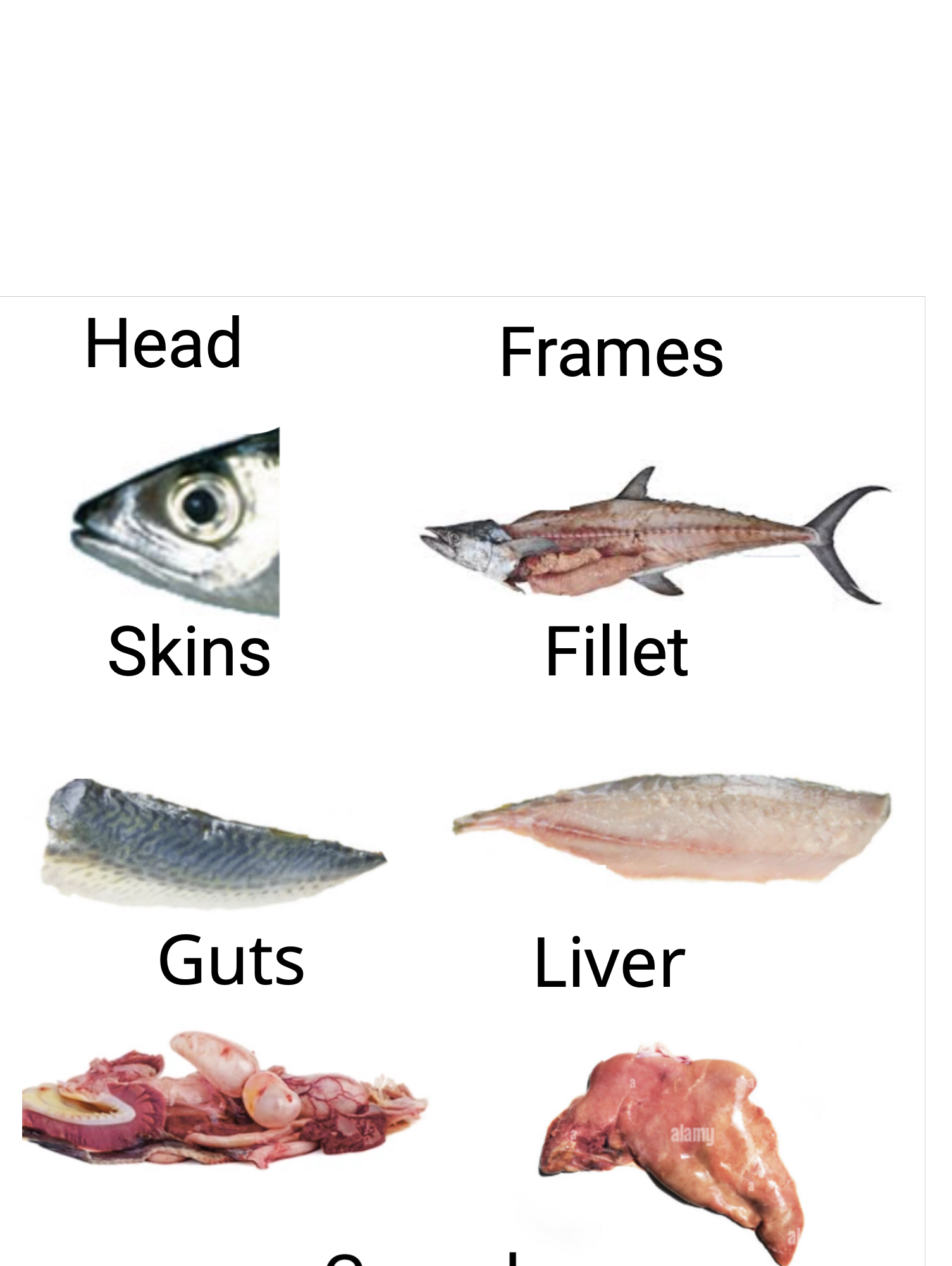
Figure 3.4: Fish body parts.
Figure 3.4: Fish body parts.
Ch. 3: Datasets and Processing
Figure 3.5: This diagram illustrates a machine learning model running on a computer to identify fish body parts. Similar
Figure 3.5: This diagram illustrates a machine learning model running on a computer to identify fish body parts. Similar
Ch. 3: Datasets and Processing
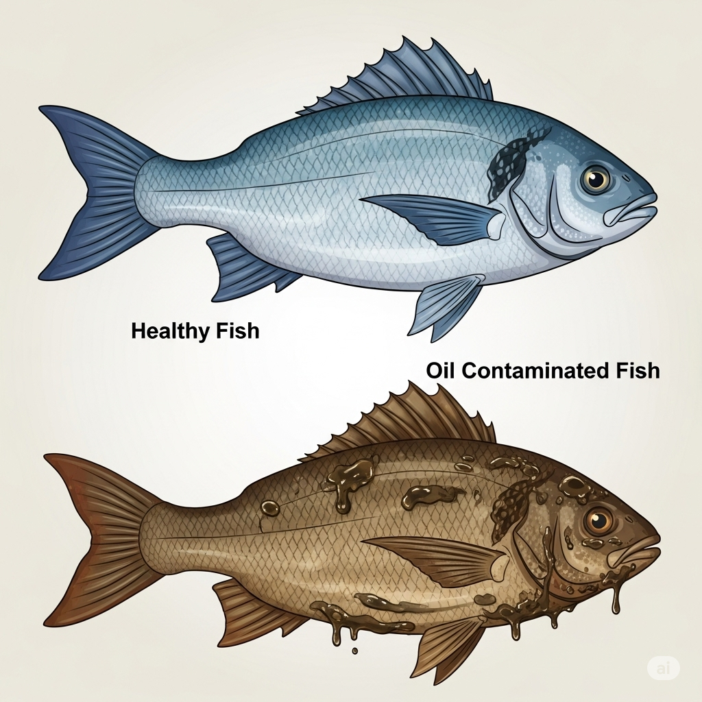
Figure 3.6: Fish are exposed to oil contamination from both human and natural sources. Major human-caused sources includ
Figure 3.6: Fish are exposed to oil contamination from both human and natural sources. Major human-caused sources includ
Ch. 3: Datasets and Processing
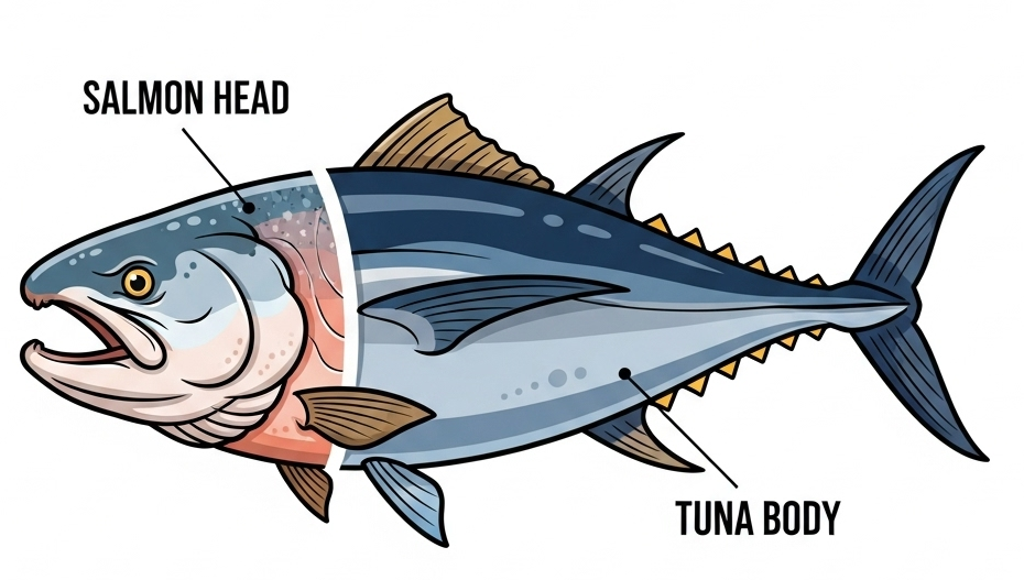
Figure 3.7: Fish can be affected by cross-species adulteration, where lower-value or unrelated species are intentionally
Figure 3.7: Fish can be affected by cross-species adulteration, where lower-value or unrelated species are intentionally
Ch. 3: Datasets and Processing
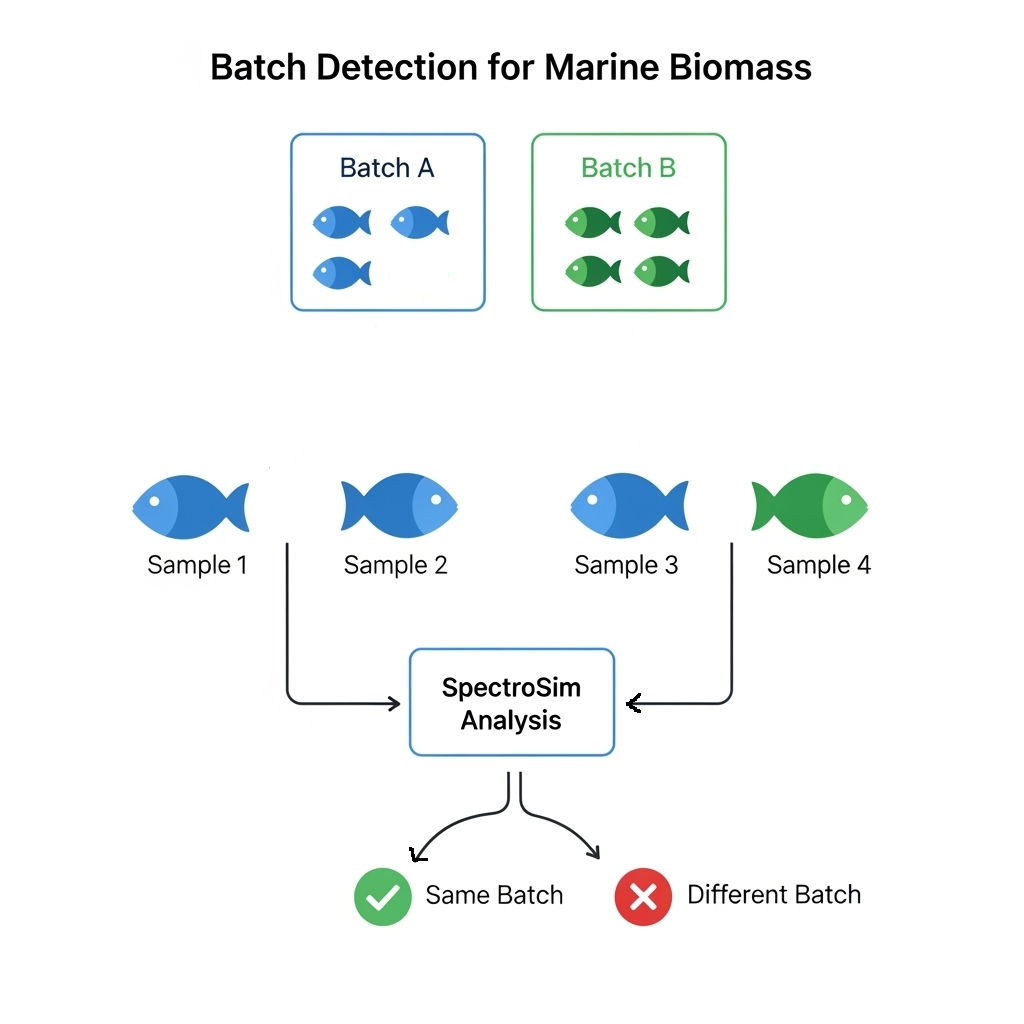
Figure 3.8: This diagram illustrates the task of batch detection for marine biomass. For simplification, we give an exam
Figure 3.8: This diagram illustrates the task of batch detection for marine biomass. For simplification, we give an exam
Ch. 4: Fish Species and Part Identifi
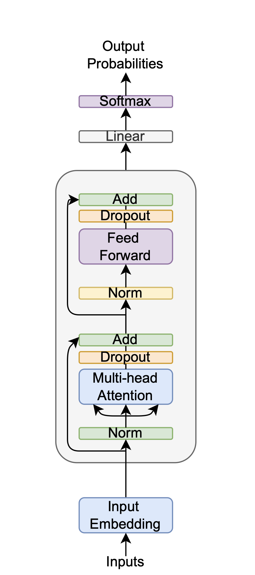
Figure 4.1: This is the transformer architecture proposed in this thesis. It is an encoder-only architecture , with four
Figure 4.1: This is the transformer architecture proposed in this thesis. It is an encoder-only architecture , with four
Ch. 4: Fish Species and Part Identifi
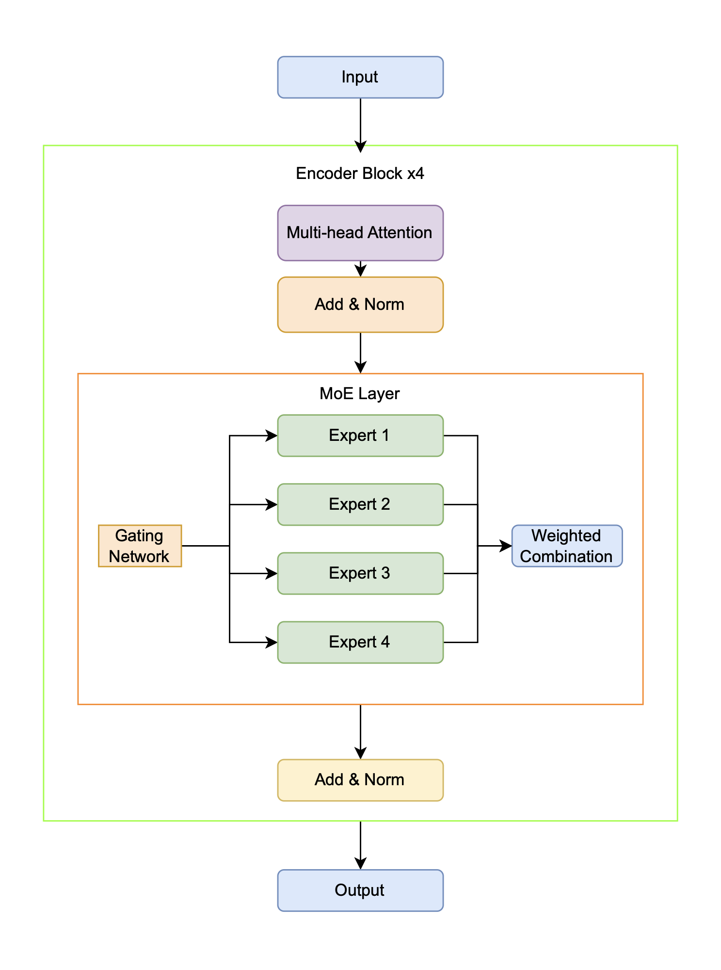
Figure 4.2: This is the MoE Transformer architecture proposed in this thesis. It consists of an encoder-only architectu
Figure 4.2: This is the MoE Transformer architecture proposed in this thesis. It consists of an encoder-only architectu
Ch. 4: Fish Species and Part Identifi
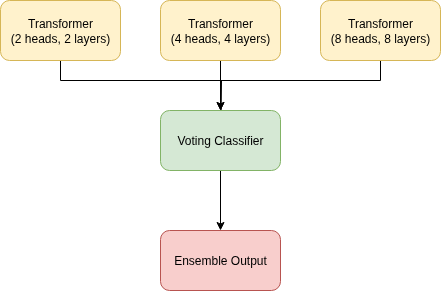
Figure 4.3: This figure shows the architecture for the stacked voting ensemble classifier, simply referred to here as th
Figure 4.3: This figure shows the architecture for the stacked voting ensemble classifier, simply referred to here as th
Ch. 4: Fish Species and Part Identifi
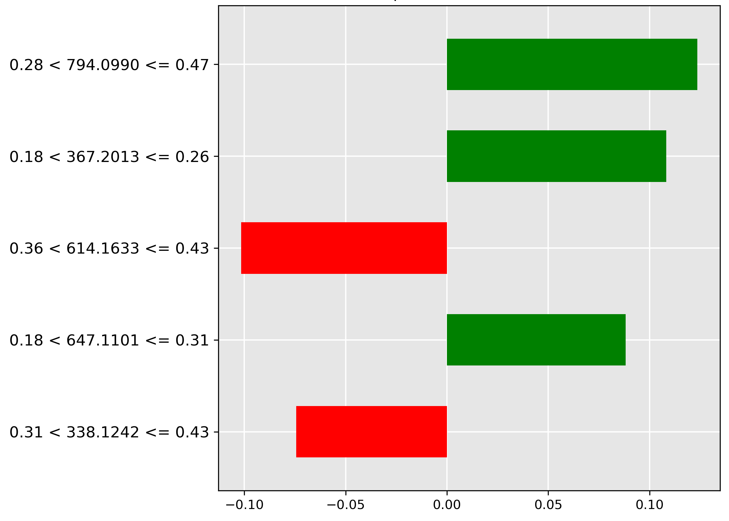
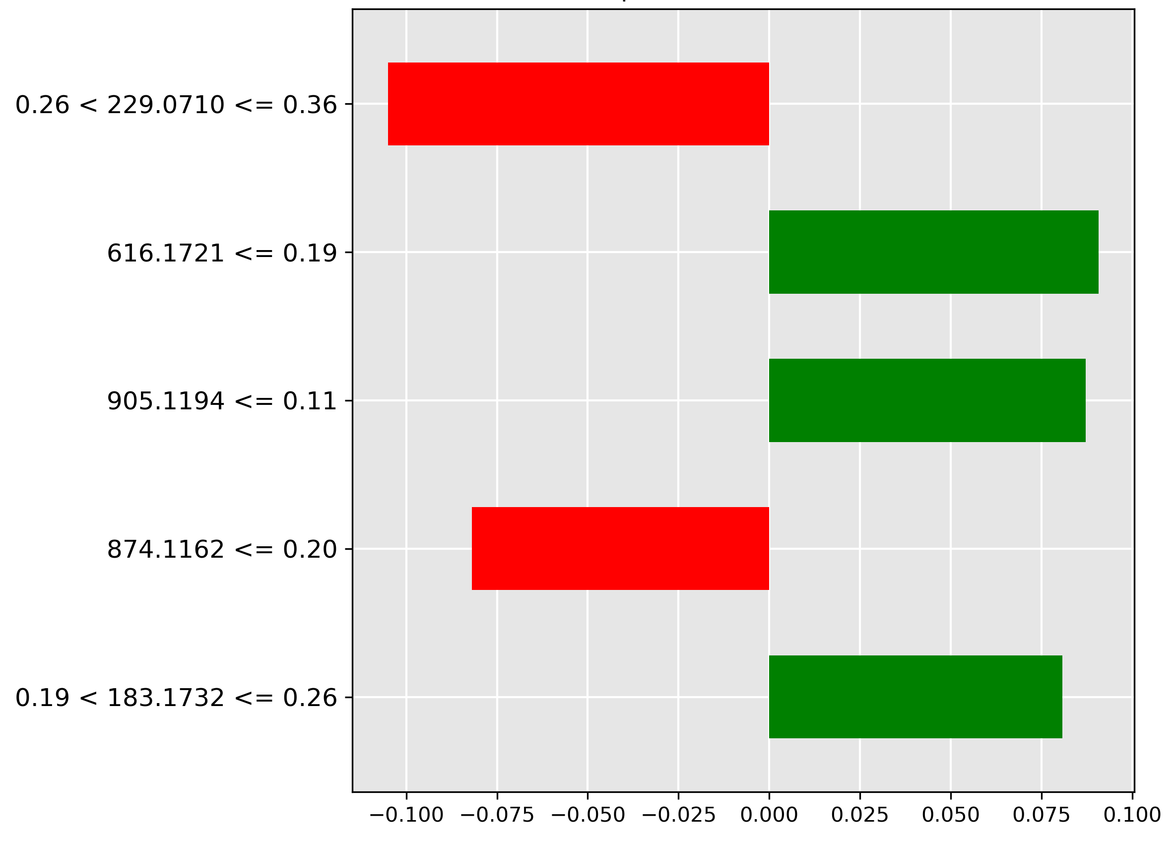
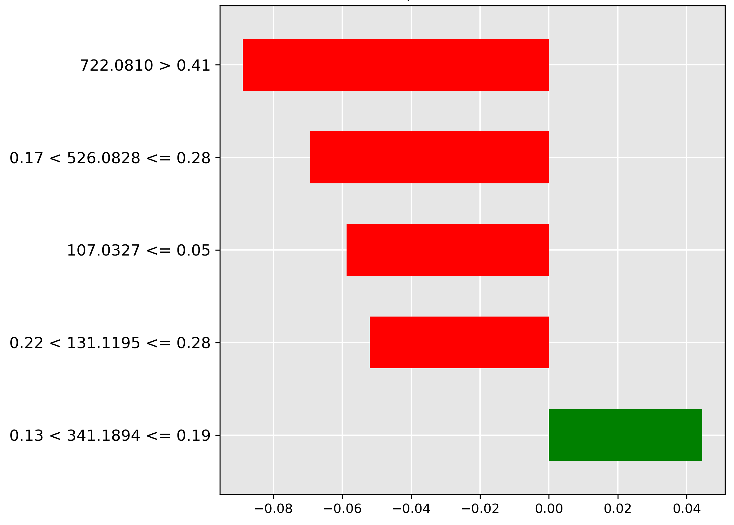
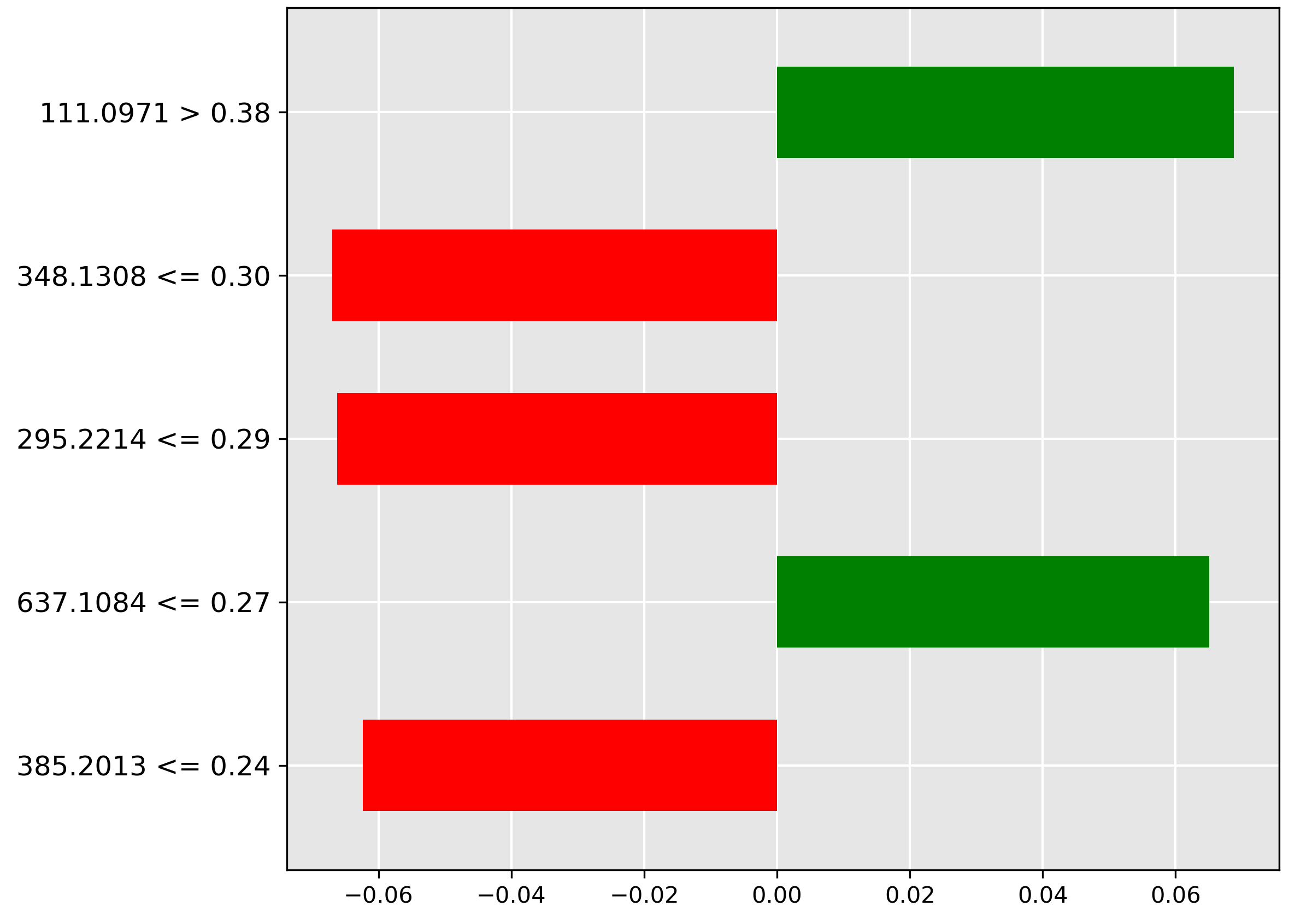
Figure 4.4: LIME explanation for pre-trained transformer for classification of fish species Mackerel.
Figure 4.4: LIME explanation for pre-trained transformer for classification of fish species Mackerel.
Ch. 4: Fish Species and Part Identifi
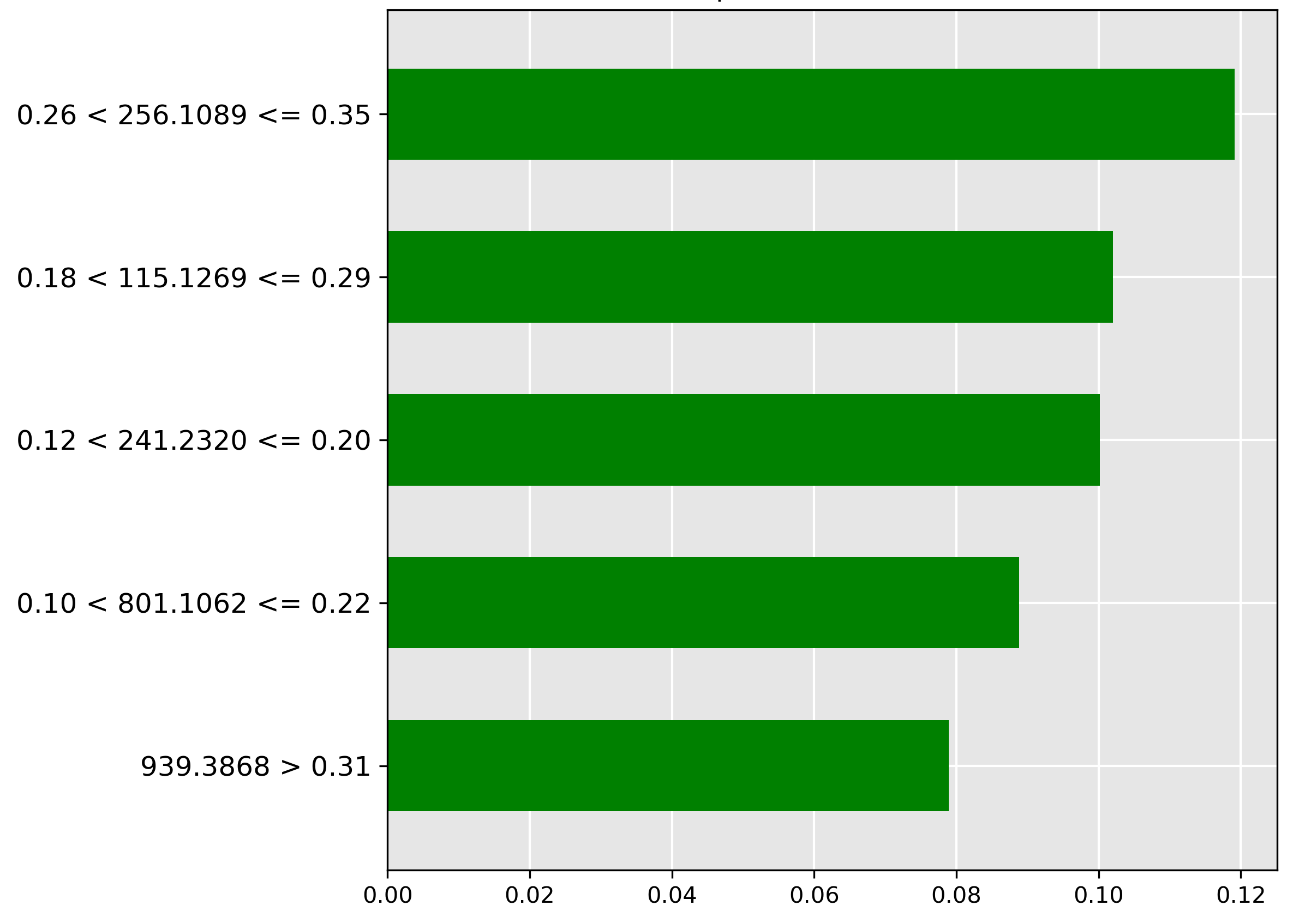
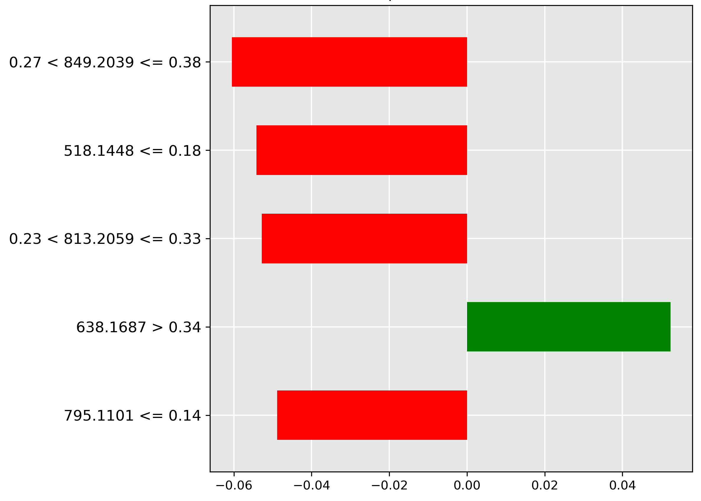
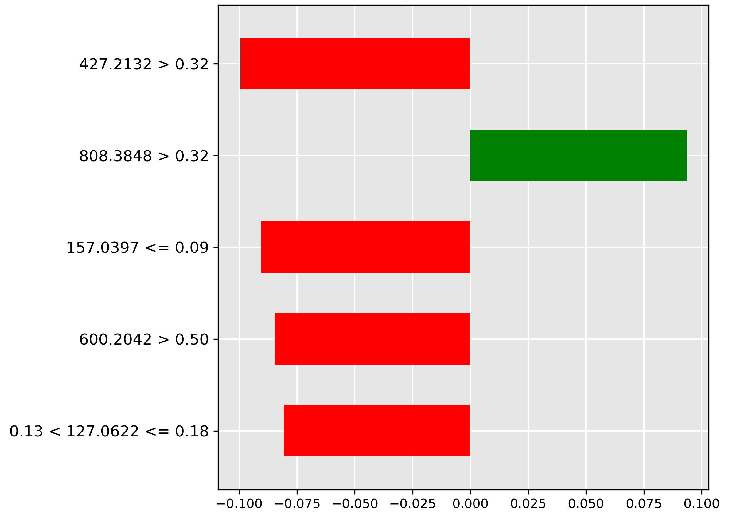
Figure 4.5: LIME explanation for pre-trained transformer for classification of fish species Hoki.
Figure 4.5: LIME explanation for pre-trained transformer for classification of fish species Hoki.
Ch. 4: Fish Species and Part Identifi
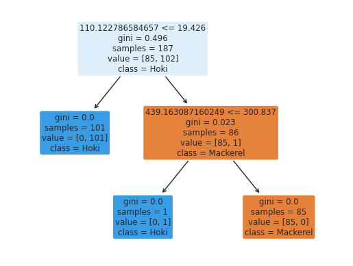
Figure 4.6: Decision tree for fish species.
Figure 4.6: Decision tree for fish species.
Ch. 4: Fish Species and Part Identifi
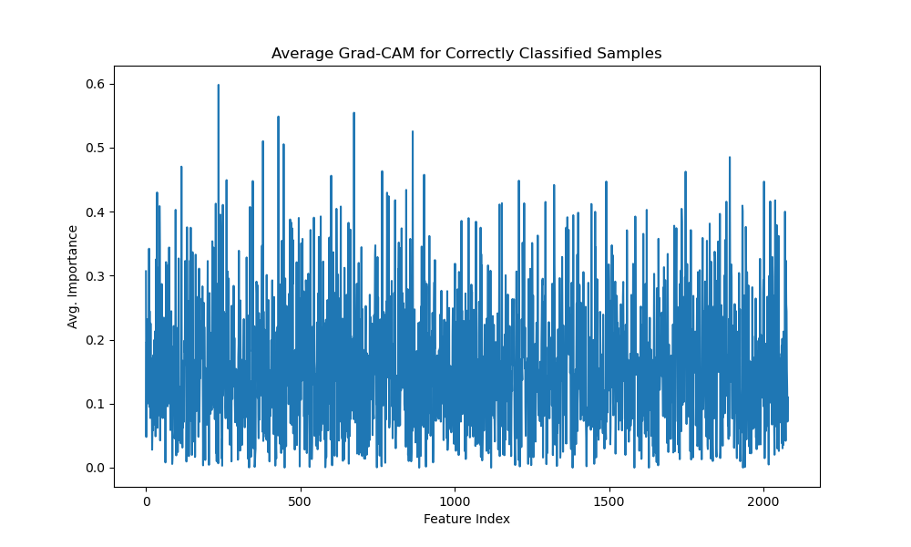
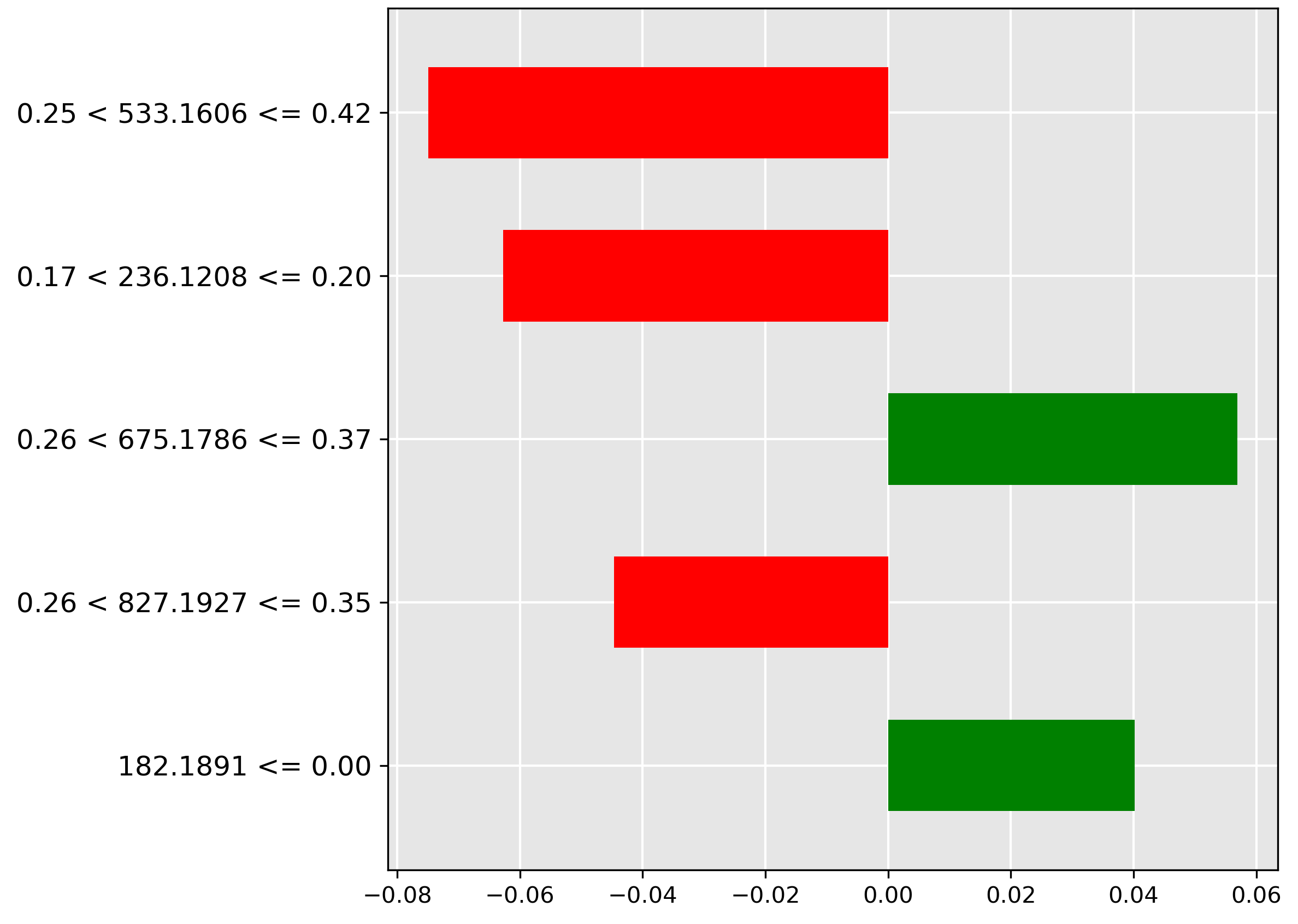
Figure 4.7: Grad-CAM for pre-trained transformer for classification of fish species.
Figure 4.7: Grad-CAM for pre-trained transformer for classification of fish species.
Ch. 4: Fish Species and Part Identifi
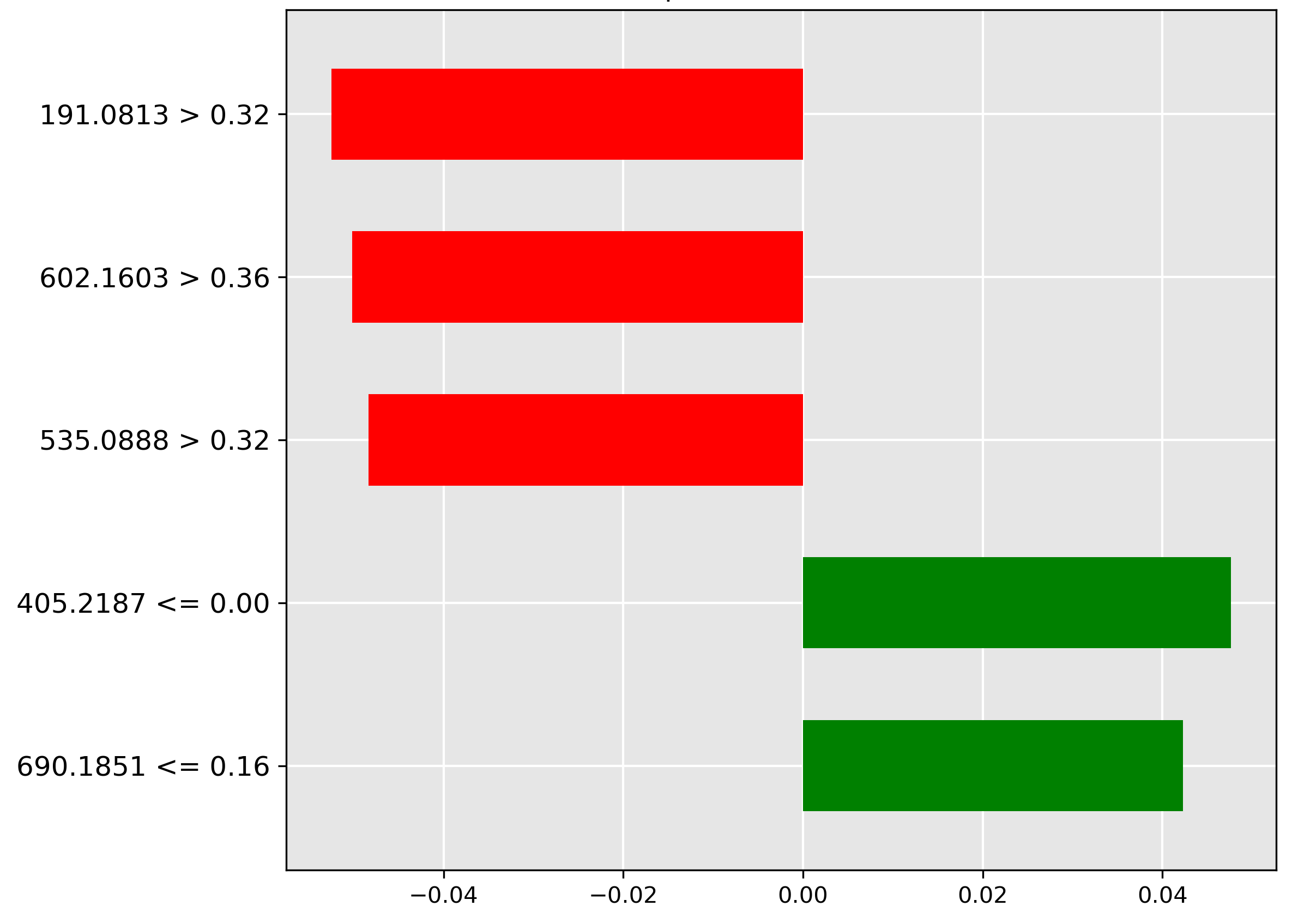
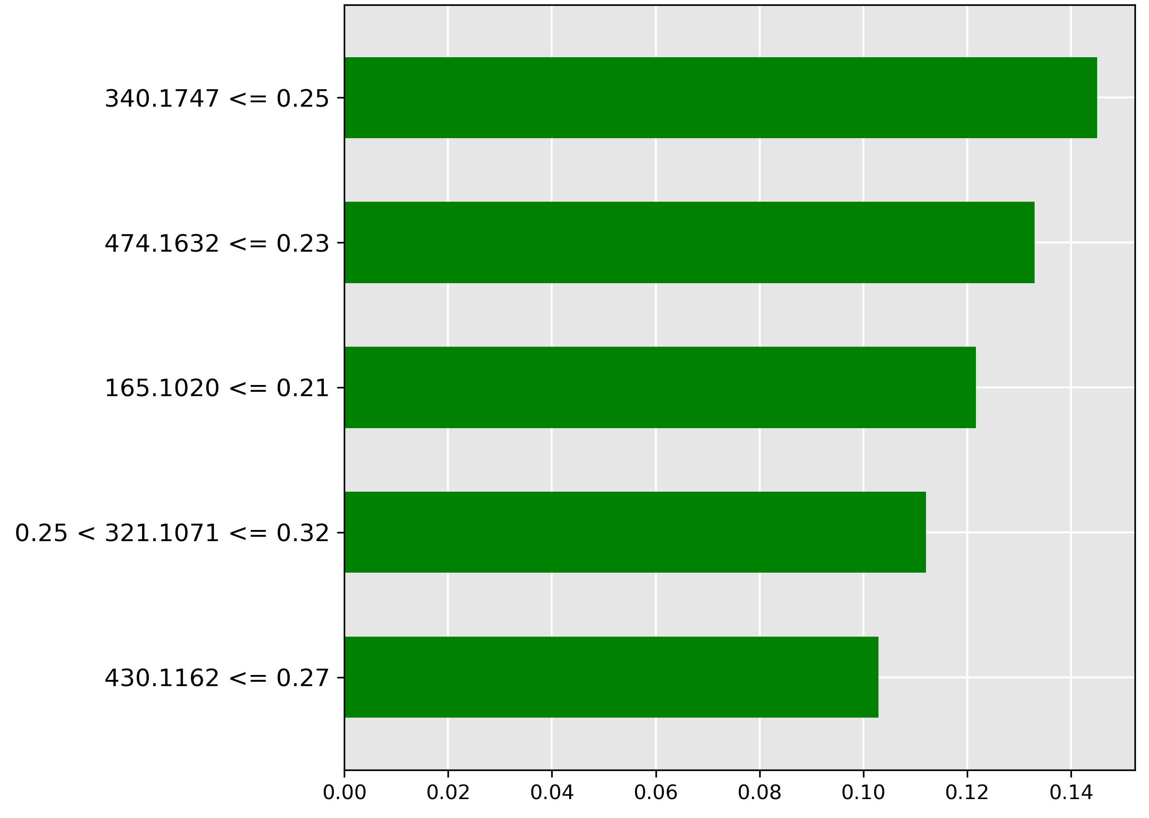
Figure 4.8: LIME explanation for transformer for classification of fish part head.
Figure 4.8: LIME explanation for transformer for classification of fish part head.
Ch. 4: Fish Species and Part Identifi
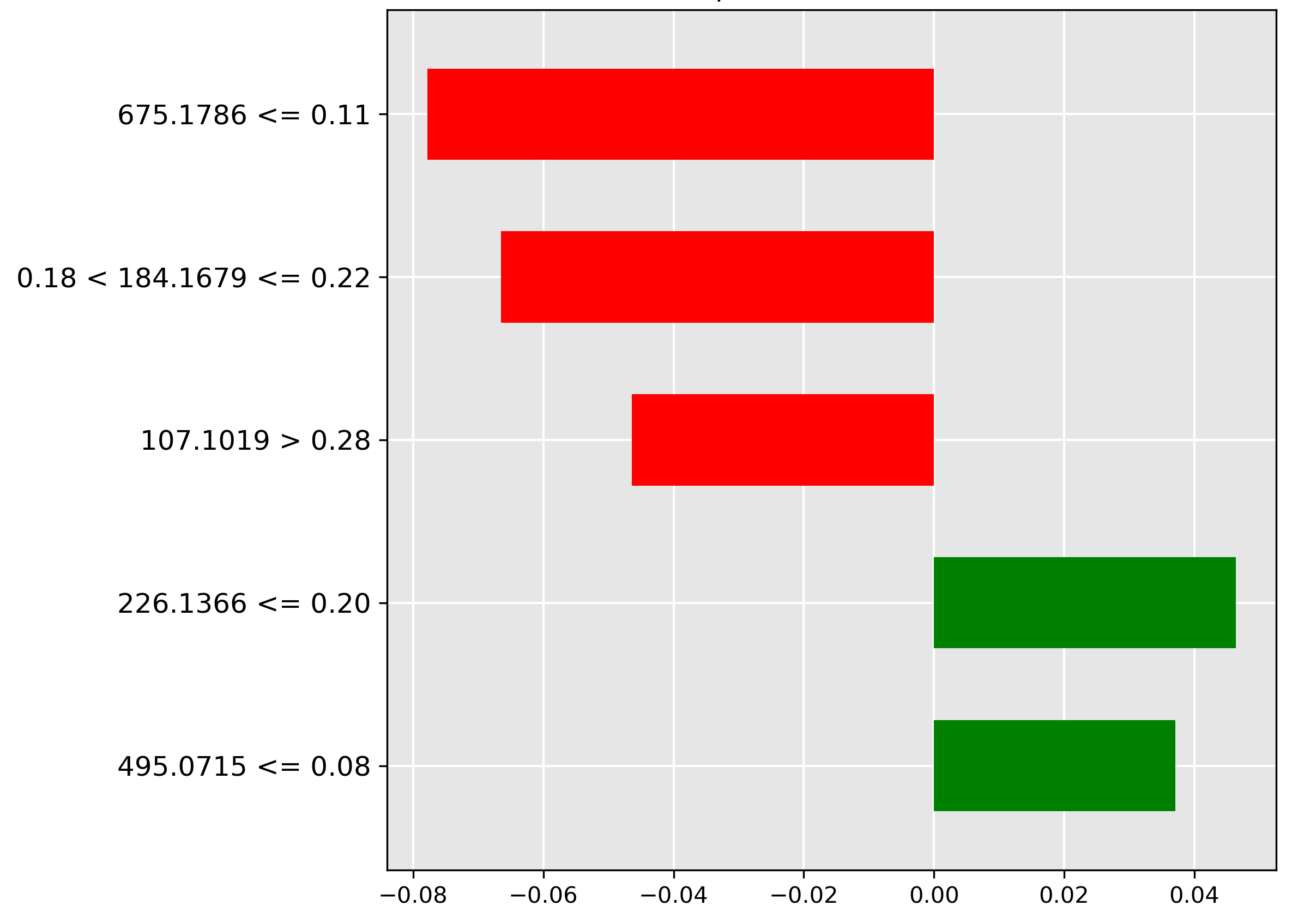
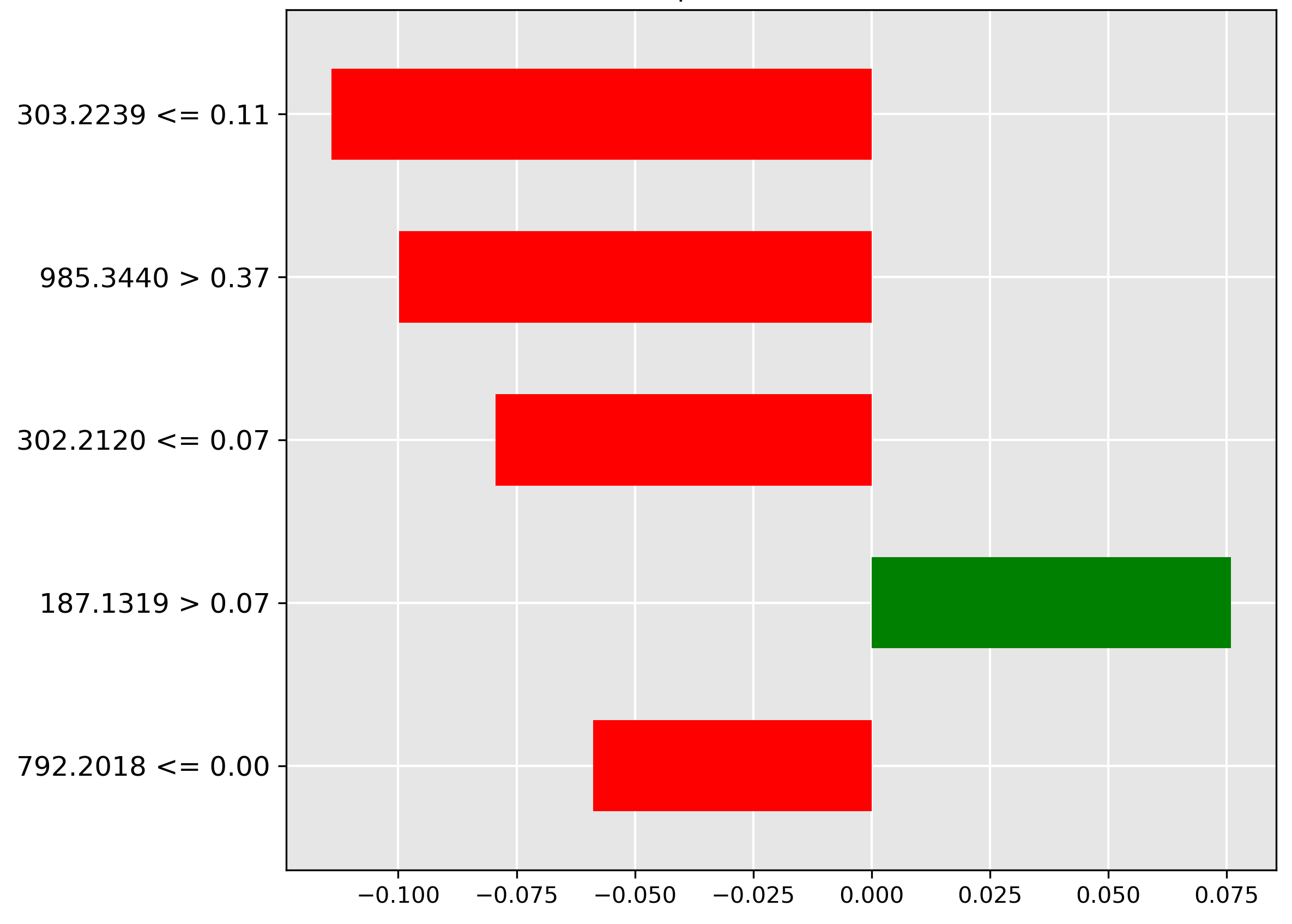
Figure 4.9: LIME explanation for transformer for classification of fish part fillet.
Figure 4.9: LIME explanation for transformer for classification of fish part fillet.
Ch. 4: Fish Species and Part Identifi
Figure 4.10: LIME explanation for transformer for classification of fish part liver.
Figure 4.10: LIME explanation for transformer for classification of fish part liver.
Ch. 4: Fish Species and Part Identifi
Figure 4.11: LIME explanation for transformer for classification of fish part skins.
Figure 4.11: LIME explanation for transformer for classification of fish part skins.
Ch. 4: Fish Species and Part Identifi
Figure 4.12: LIME explanation for transformer for classification of fish part guts.
Figure 4.12: LIME explanation for transformer for classification of fish part guts.
Ch. 4: Fish Species and Part Identifi
Figure 4.13: LIME explanation for transformer for classification of fish part frames.
Figure 4.13: LIME explanation for transformer for classification of fish part frames.
Ch. 4: Fish Species and Part Identifi
Figure 4.14: LIME explanation for transformer for classification of fish part gonads.
Figure 4.14: LIME explanation for transformer for classification of fish part gonads.
Ch. 4: Fish Species and Part Identifi
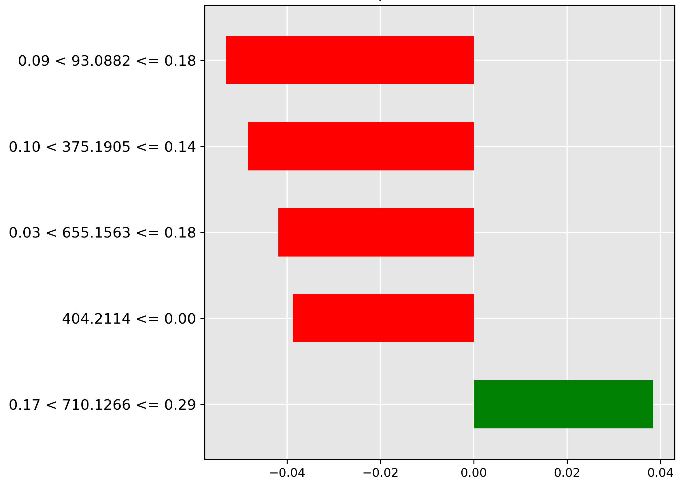
Figure 4.15: Grad-CAM for transformer for classification of fish body part.
Figure 4.15: Grad-CAM for transformer for classification of fish body part.
Ch. 4: Fish Species and Part Identifi
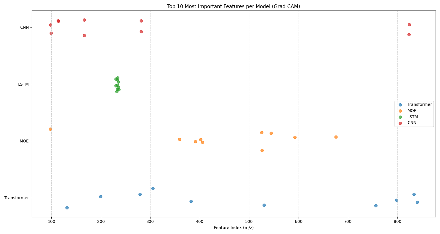
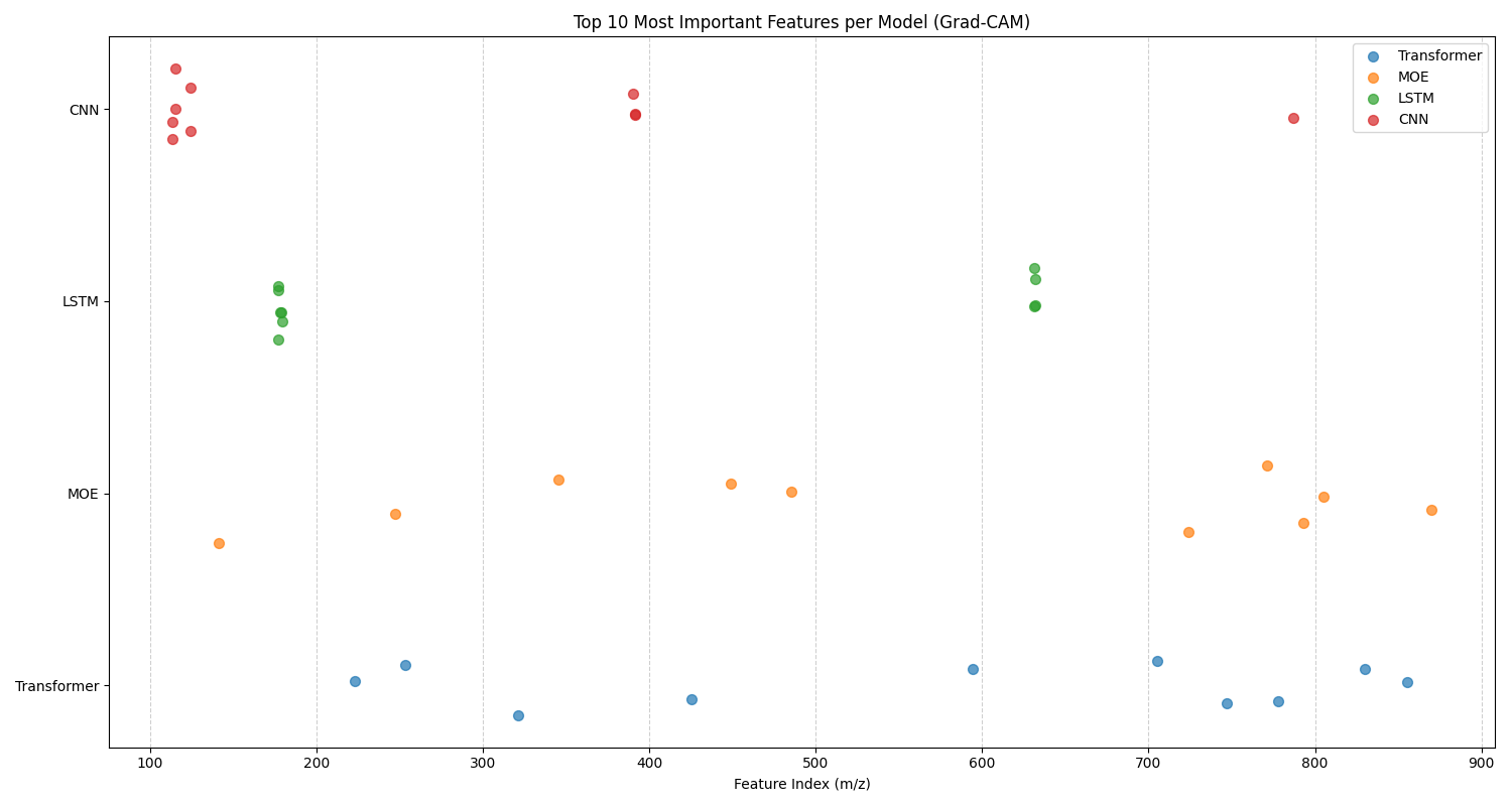
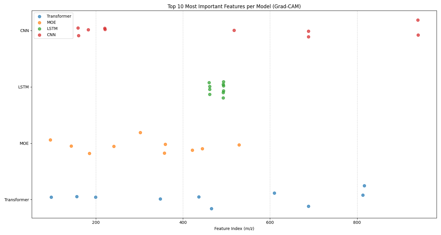
Figure 4.16: In this diagram, we present the top 10 features for fish species classification for each method that have b
Figure 4.16: In this diagram, we present the top 10 features for fish species classification for each method that have b
Ch. 4: Fish Species and Part Identifi
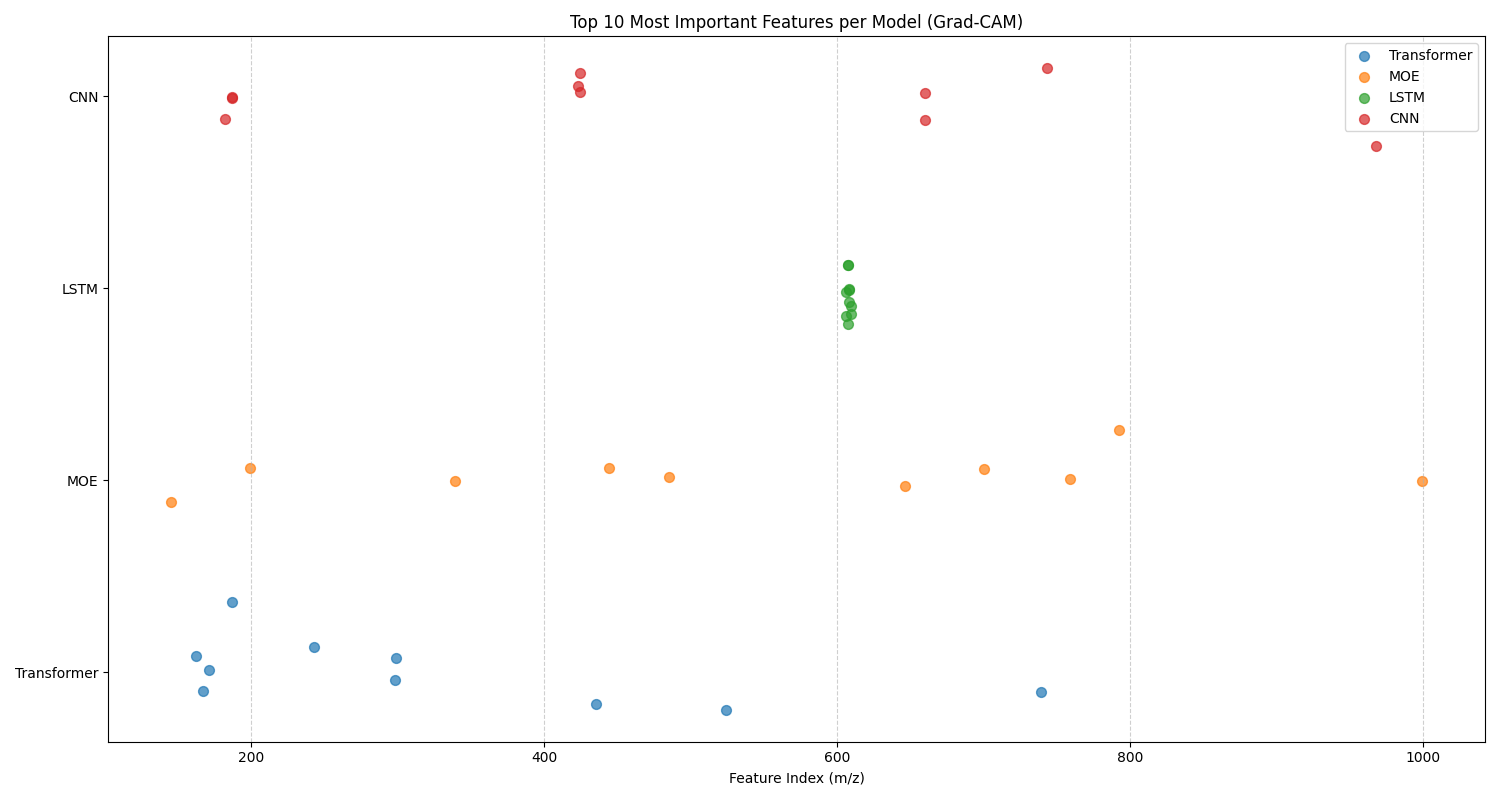
Figure 4.17: In this diagram, we present the top 10 features for fish part classification for each method that have been
Figure 4.17: In this diagram, we present the top 10 features for fish part classification for each method that have been
Ch. 4: Fish Species and Part Identifi
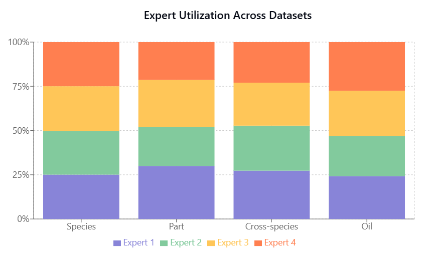
Figure 4.18: This stacked bar chart shows the expert utilization of the MoE Transformer with 4 experts across all four c
Figure 4.18: This stacked bar chart shows the expert utilization of the MoE Transformer with 4 experts across all four c
Ch. 4: Fish Species and Part Identifi
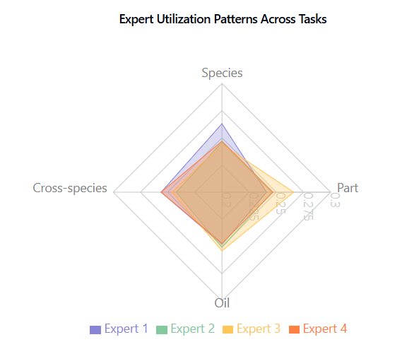
Figure 4.19: This radar chart illustrates the utilization patterns of four different experts across four task categories
Figure 4.19: This radar chart illustrates the utilization patterns of four different experts across four task categories
Ch. 4: Fish Species and Part Identifi
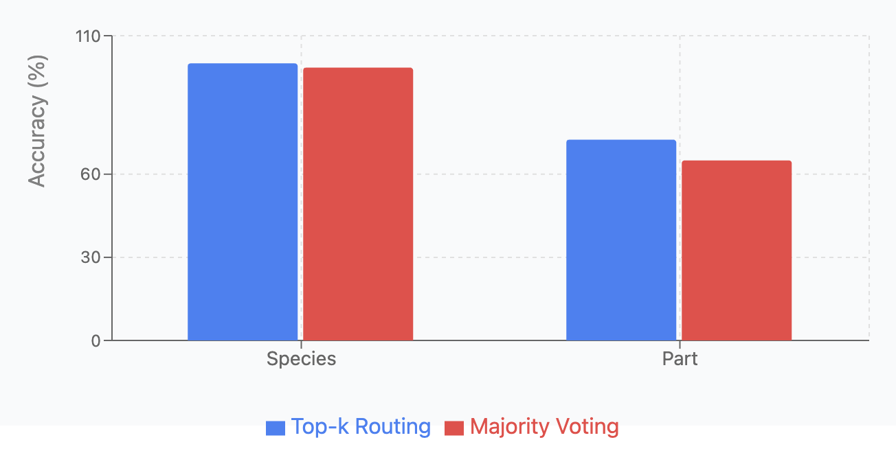
Figure 4.20: Majority Voting versus Top-k Routing Bar Chart. This chart gives the test classification accuracy on the fi
Figure 4.20: Majority Voting versus Top-k Routing Bar Chart. This chart gives the test classification accuracy on the fi
Ch. 4: Fish Species and Part Identifi
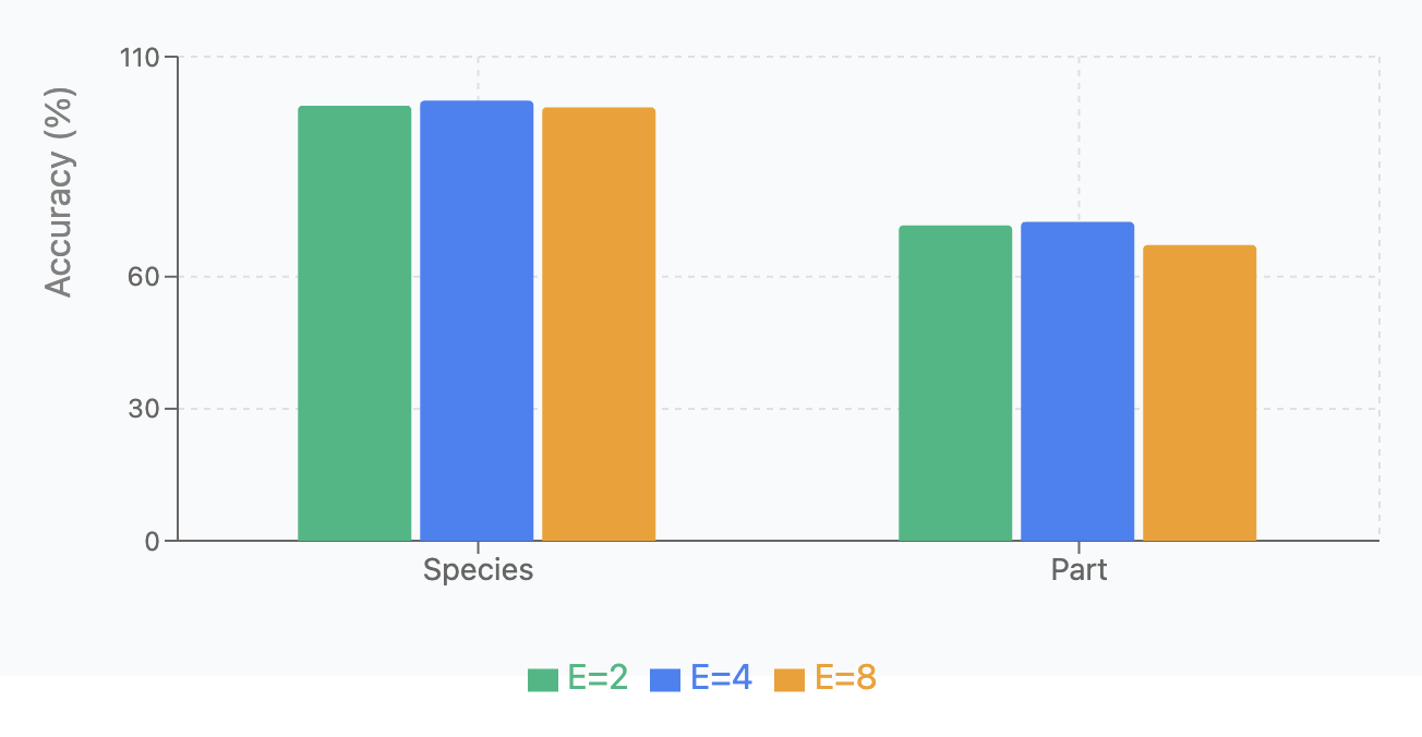
Figure 4.21: Expert Count Analysis Bar Chart. This bar chart illustrates the test classification accuracy across the two
Figure 4.21: Expert Count Analysis Bar Chart. This bar chart illustrates the test classification accuracy across the two
Ch. 4: Fish Species and Part Identifi
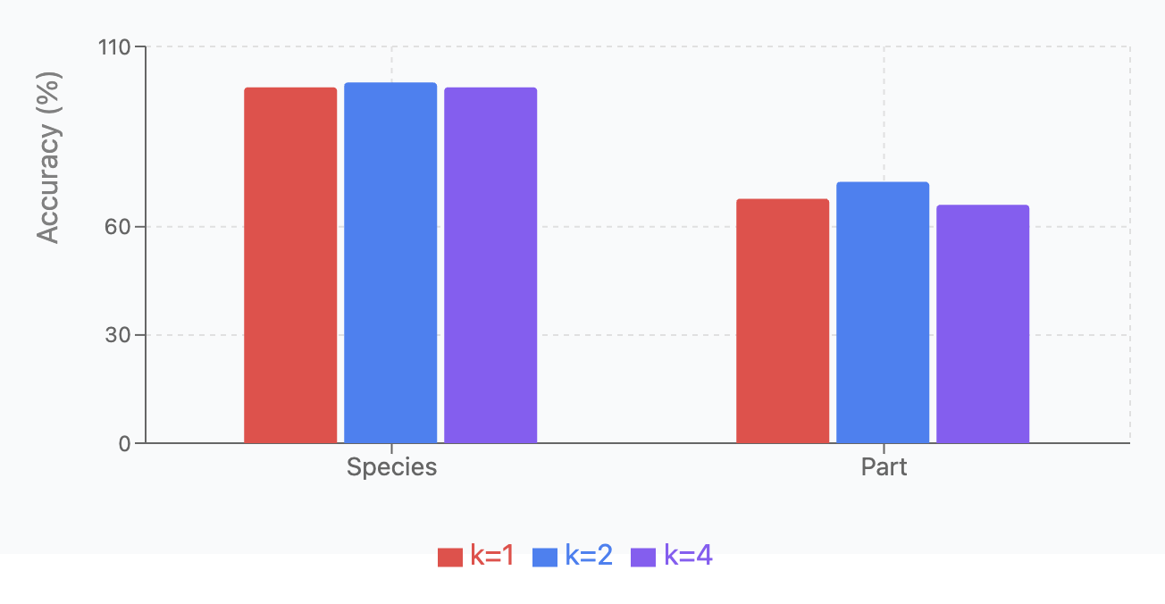
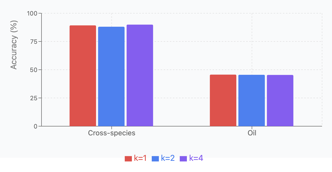
Figure 4.22: Top-k Routing Bar Chart. This bar chart illustrates the test classification accuracy for the two tasks of f
Figure 4.22: Top-k Routing Bar Chart. This bar chart illustrates the test classification accuracy for the two tasks of f
Ch. 5: Oil Contamination and Cross-Sp
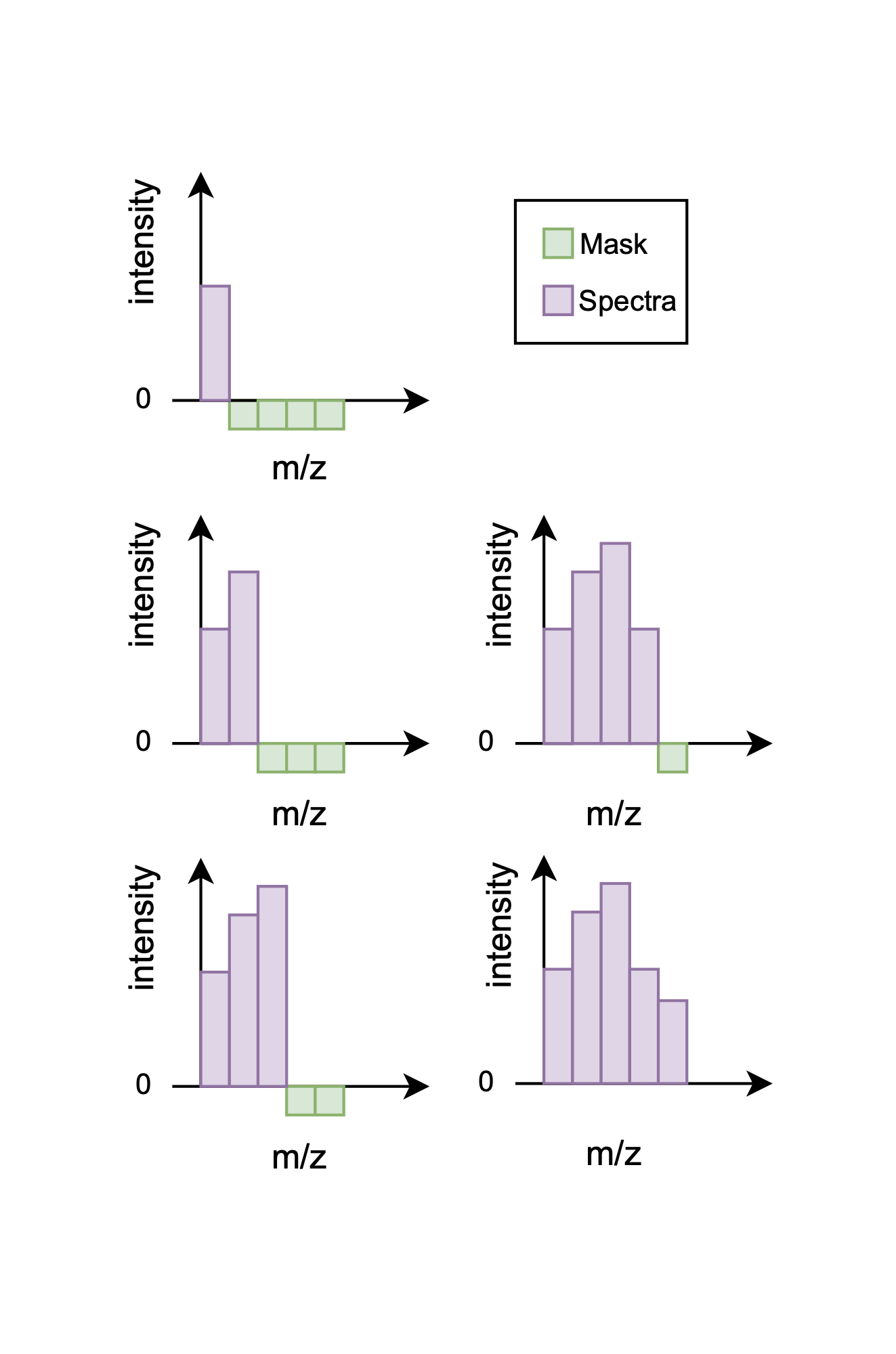
Figure 5.1: Masked Spectra Modelling is a variation of Masked Language Modeling from BERT . But unlike BERT, which uses
Figure 5.1: Masked Spectra Modelling is a variation of Masked Language Modeling from BERT . But unlike BERT, which uses
Ch. 5: Oil Contamination and Cross-Sp
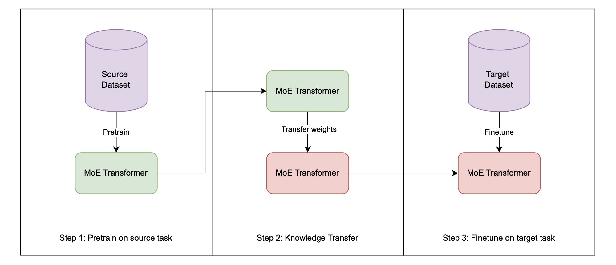
Figure 5.2: Transfer Learning Overview: The image outlines the transfer learning workflow with MoE Transformers. Step 1
Figure 5.2: Transfer Learning Overview: The image outlines the transfer learning workflow with MoE Transformers. Step 1
Ch. 5: Oil Contamination and Cross-Sp
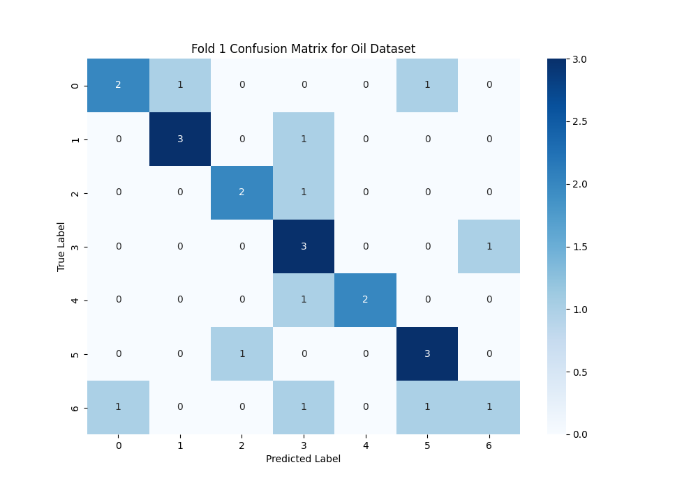
Figure 5.3: The confusion matrix on the test dataset for one of the folds of cross-validation. The diagonal of the matri
Figure 5.3: The confusion matrix on the test dataset for one of the folds of cross-validation. The diagonal of the matri
Ch. 5: Oil Contamination and Cross-Sp
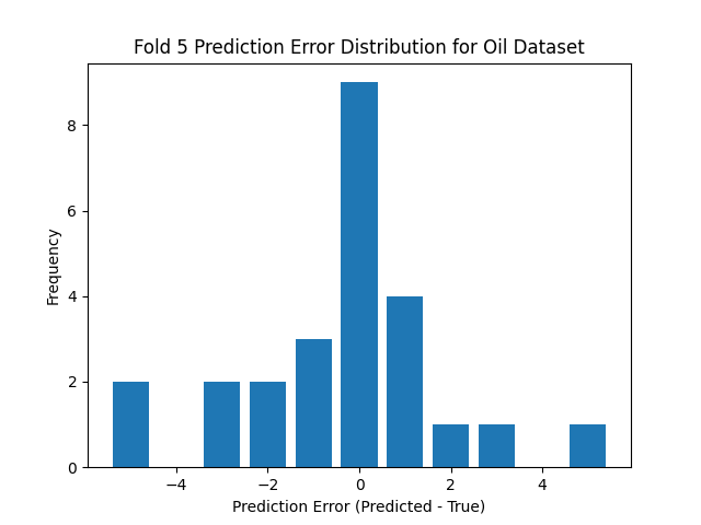
Figure 5.4: The prediction error histogram denotes how far off each of the predictions was. Since this is an ordinal cla
Figure 5.4: The prediction error histogram denotes how far off each of the predictions was. Since this is an ordinal cla
Ch. 5: Oil Contamination and Cross-Sp
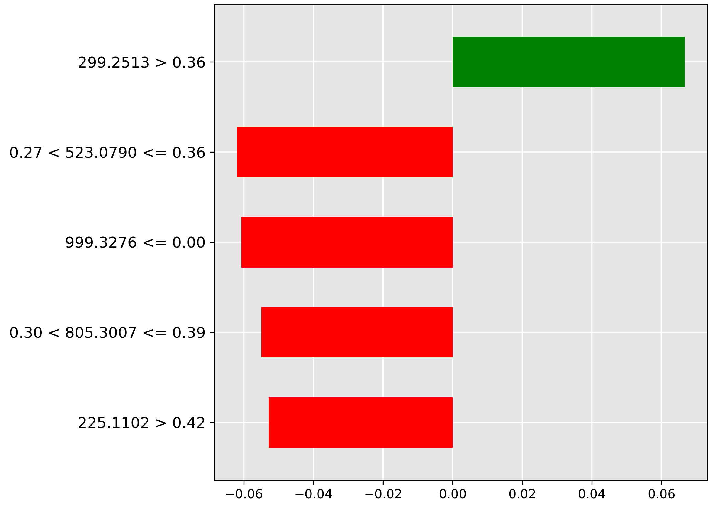
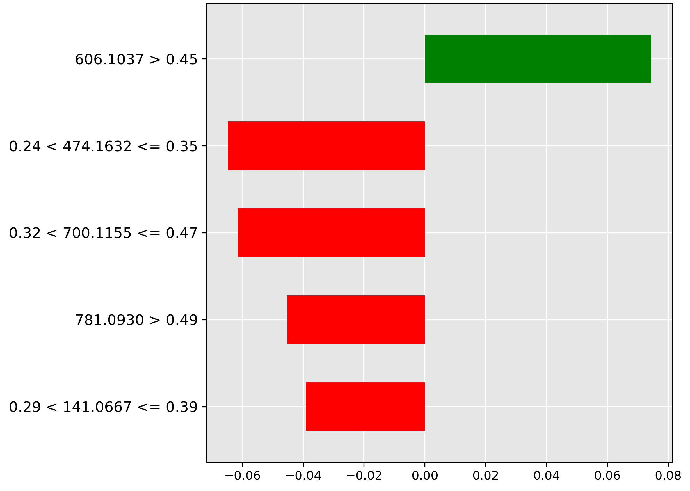
Figure 5.5: LIME explanation for pre-trained transformer for classification of oil contamination in 50\% concentration.
Figure 5.5: LIME explanation for pre-trained transformer for classification of oil contamination in 50\% concentration.
Ch. 5: Oil Contamination and Cross-Sp
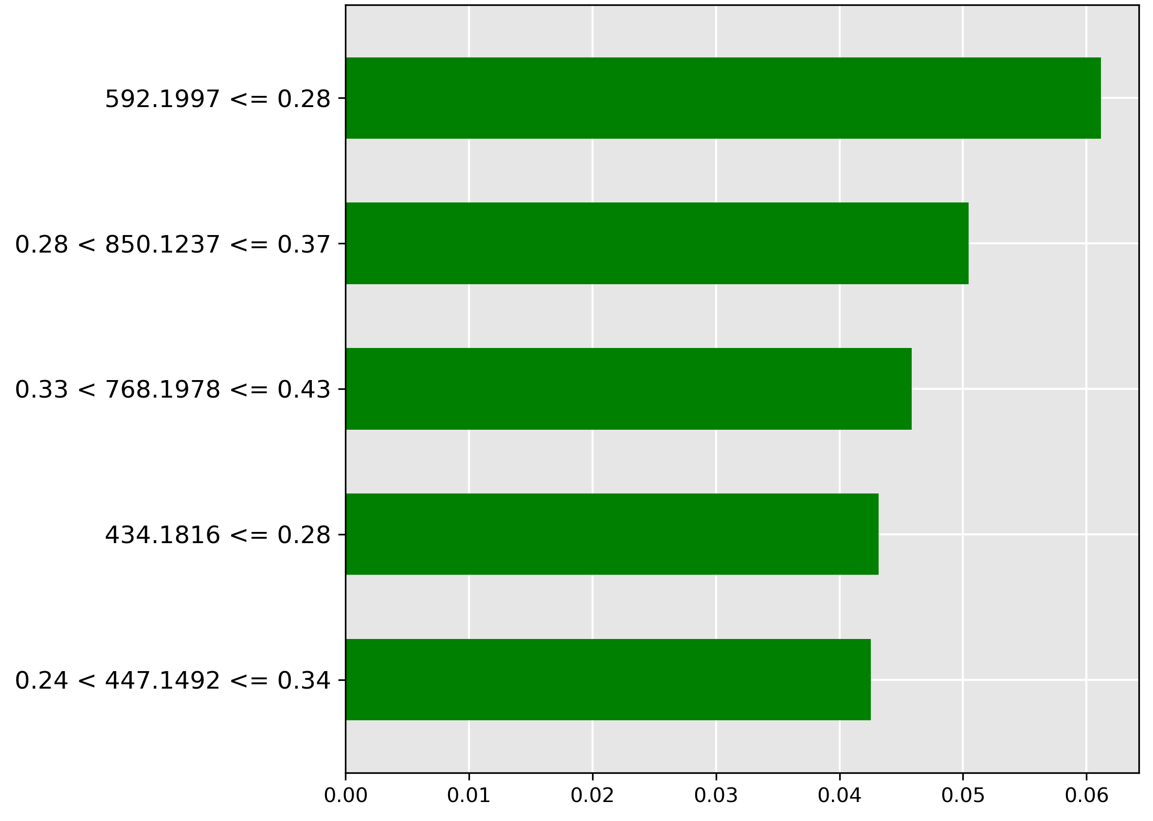
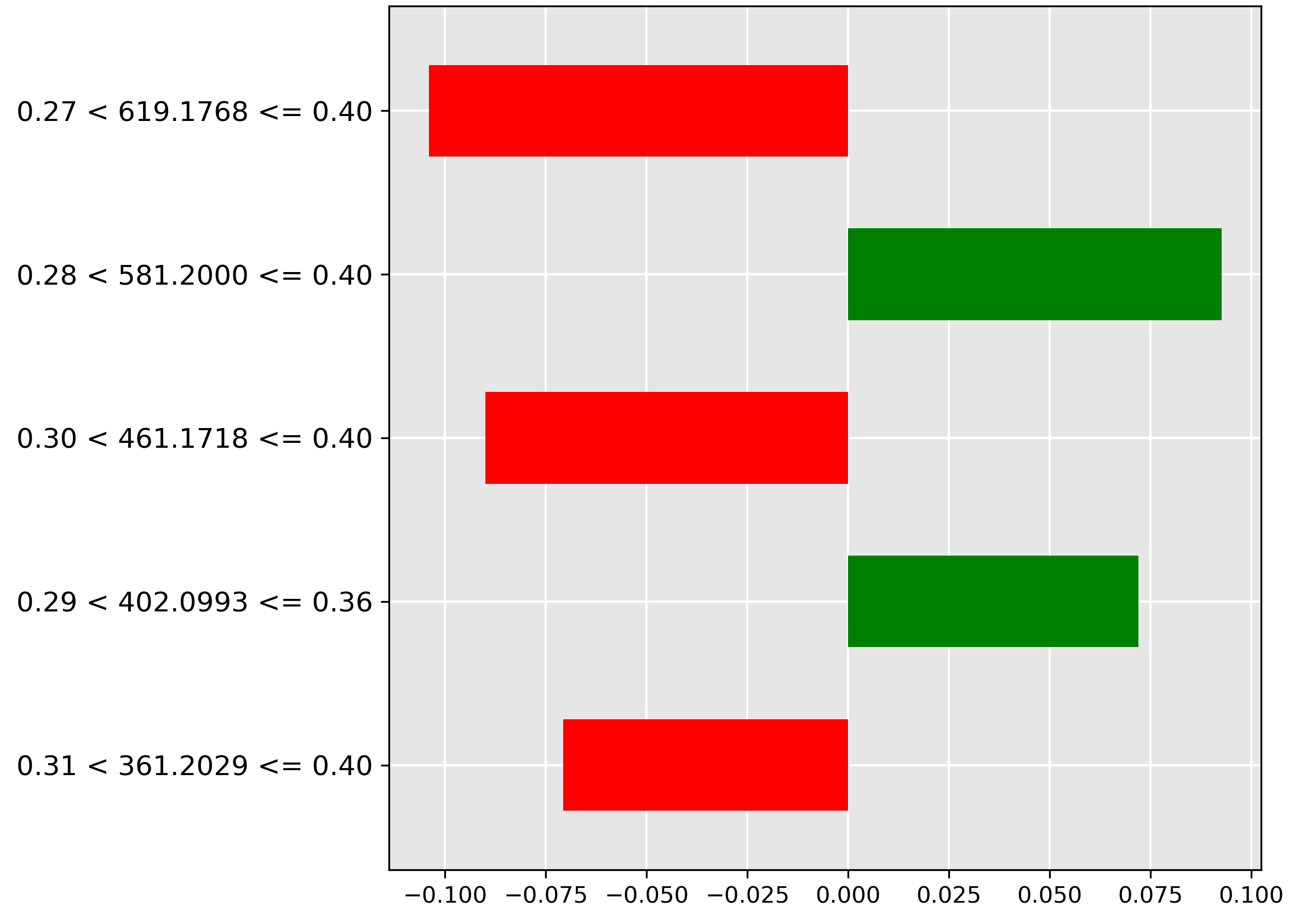
Figure 5.6: LIME explanation for pre-trained transformer for classification of oil contamination in 25\% concentration.
Figure 5.6: LIME explanation for pre-trained transformer for classification of oil contamination in 25\% concentration.
Ch. 5: Oil Contamination and Cross-Sp
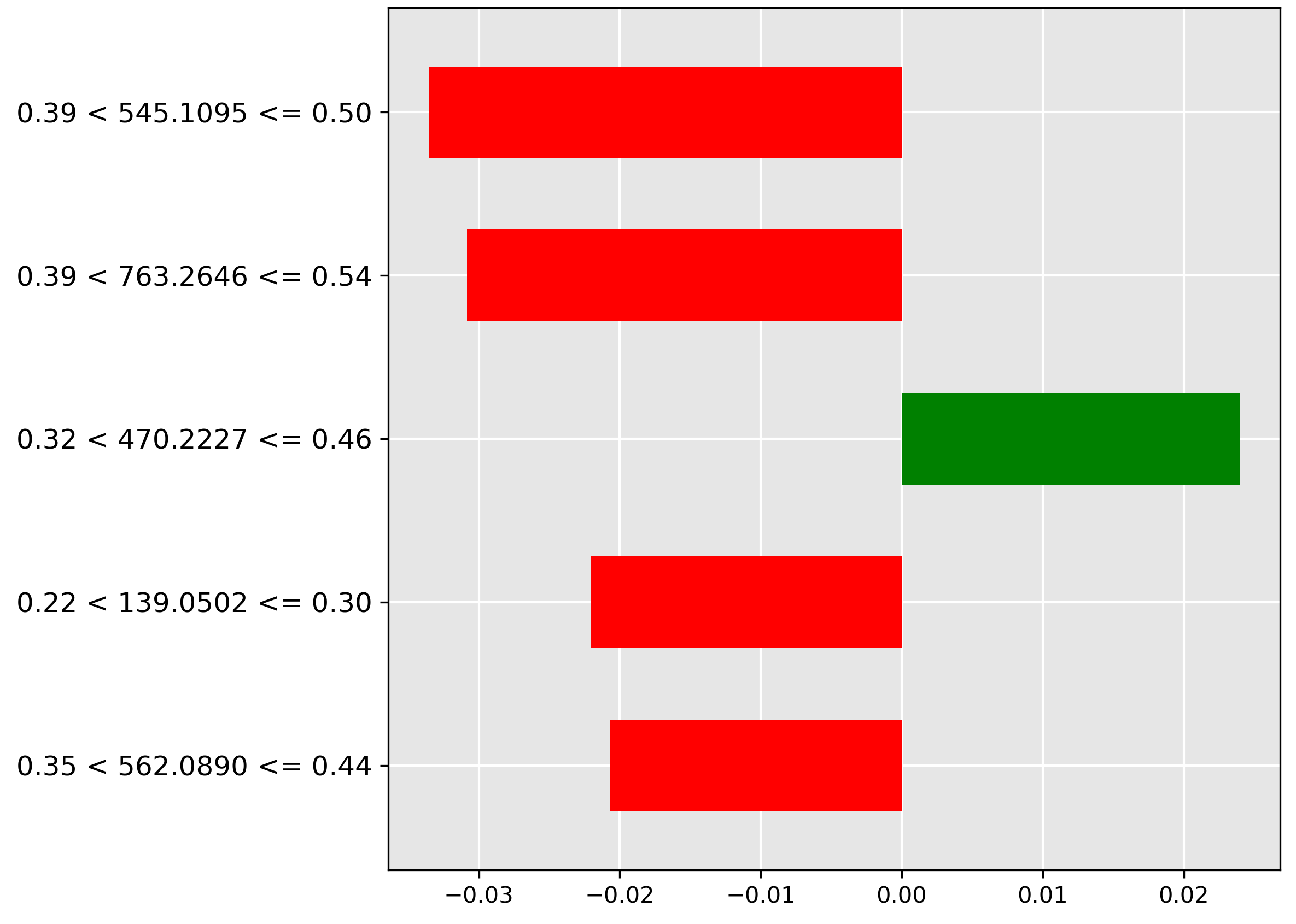
Figure 5.7: LIME explanation for pre-trained transformer for classification of oil contamination in 10\% concentration.
Figure 5.7: LIME explanation for pre-trained transformer for classification of oil contamination in 10\% concentration.
Ch. 5: Oil Contamination and Cross-Sp
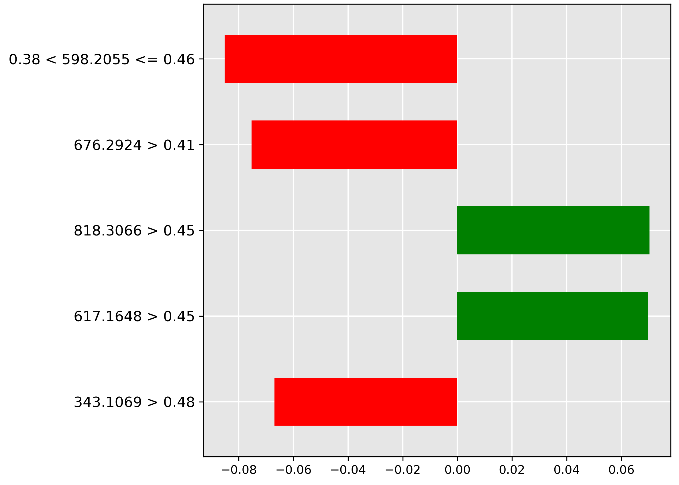
Figure 5.8: LIME explanation for pre-trained transformer for classification of oil contamination in 5\% concentration.
Figure 5.8: LIME explanation for pre-trained transformer for classification of oil contamination in 5\% concentration.
Ch. 5: Oil Contamination and Cross-Sp
Figure 5.9: LIME explanation for pre-trained transformer for classification of oil contamination in 1\% concentration.
Figure 5.9: LIME explanation for pre-trained transformer for classification of oil contamination in 1\% concentration.
Ch. 5: Oil Contamination and Cross-Sp
Figure 5.10: LIME explanation for pre-trained transformer for classification of oil contamination in 0.1\% concentration
Figure 5.10: LIME explanation for pre-trained transformer for classification of oil contamination in 0.1\% concentration
Ch. 5: Oil Contamination and Cross-Sp
Figure 5.11: LIME explanation for pre-trained transformer for classification of oil contamination in 0\% concentration.
Figure 5.11: LIME explanation for pre-trained transformer for classification of oil contamination in 0\% concentration.
Ch. 5: Oil Contamination and Cross-Sp
Figure 5.12: LIME explanation for pre-trained transformer for cross-species contamination of Hoki-Mackerel class.
Figure 5.12: LIME explanation for pre-trained transformer for cross-species contamination of Hoki-Mackerel class.
Ch. 5: Oil Contamination and Cross-Sp
Figure 5.13: LIME explanation for pre-trained transformer for cross-species contamination of Hoki class.
Figure 5.13: LIME explanation for pre-trained transformer for cross-species contamination of Hoki class.
Ch. 5: Oil Contamination and Cross-Sp
Figure 5.14: LIME explanation for pre-trained transformer for cross-species contamination of Mackerel class.
Figure 5.14: LIME explanation for pre-trained transformer for cross-species contamination of Mackerel class.
Ch. 5: Oil Contamination and Cross-Sp
Figure 5.15: In this diagram, we present the top 10 features for oil contamination classification that have been identif
Figure 5.15: In this diagram, we present the top 10 features for oil contamination classification that have been identif
Ch. 5: Oil Contamination and Cross-Sp
Figure 5.16: In this diagram, we present the top 10 features for fish cross-species adulteration classification that hav
Figure 5.16: In this diagram, we present the top 10 features for fish cross-species adulteration classification that hav
Ch. 5: Oil Contamination and Cross-Sp
Figure 5.17: This stacked bar chart shows the expert utilization of the MoE Transformer with 4 experts across all four c
Figure 5.17: This stacked bar chart shows the expert utilization of the MoE Transformer with 4 experts across all four c
Ch. 5: Oil Contamination and Cross-Sp
Figure 5.18: This radar chart illustrates the utilization patterns of four different experts across four task categories
Figure 5.18: This radar chart illustrates the utilization patterns of four different experts across four task categories
Ch. 5: Oil Contamination and Cross-Sp
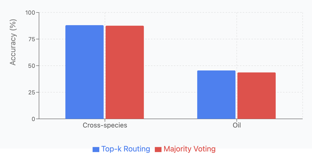
Figure 5.19: Majority Voting versus Top-k Routing Bar Chart
Figure 5.19: Majority Voting versus Top-k Routing Bar Chart
Ch. 5: Oil Contamination and Cross-Sp
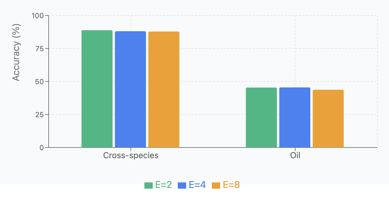
Figure 5.20: Expert Count Analysis Bar Chart
Figure 5.20: Expert Count Analysis Bar Chart
Ch. 5: Oil Contamination and Cross-Sp
Figure 5.21: Top-k Routing Bar Chart
Figure 5.21: Top-k Routing Bar Chart
Ch. 5: Oil Contamination and Cross-Sp
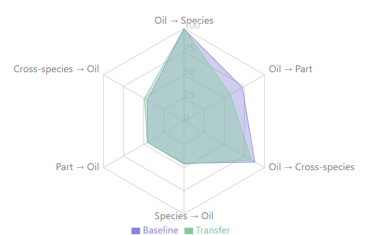
Figure 5.22: Test Classification Improvements Radar Chart: This radar chart provides a comparative view of Baseline (gre
Figure 5.22: Test Classification Improvements Radar Chart: This radar chart provides a comparative view of Baseline (gre
Ch. 5: Oil Contamination and Cross-Sp
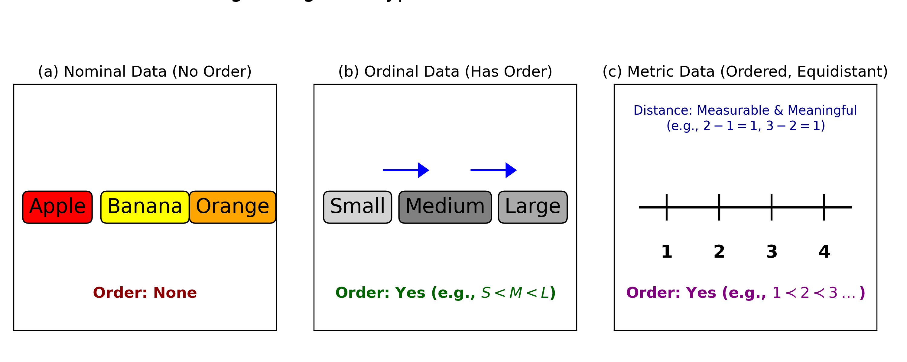
Figure 5.23: A conceptual comparison of data measurement scales, illustrating the unique nature of (b) Ordinal Data, whe
Figure 5.23: A conceptual comparison of data measurement scales, illustrating the unique nature of (b) Ordinal Data, whe
Ch. 5: Oil Contamination and Cross-Sp
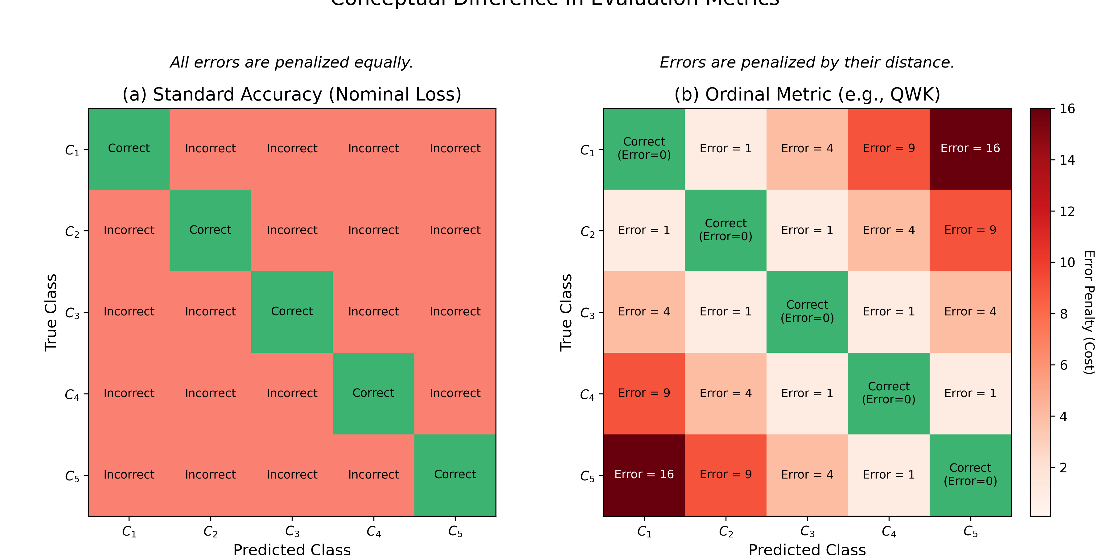
Figure 5.24: Conceptual difference in evaluation. (a) Standard accuracy treats all misclassifications as equally incorre
Figure 5.24: Conceptual difference in evaluation. (a) Standard accuracy treats all misclassifications as equally incorre
Ch. 5: Oil Contamination and Cross-Sp
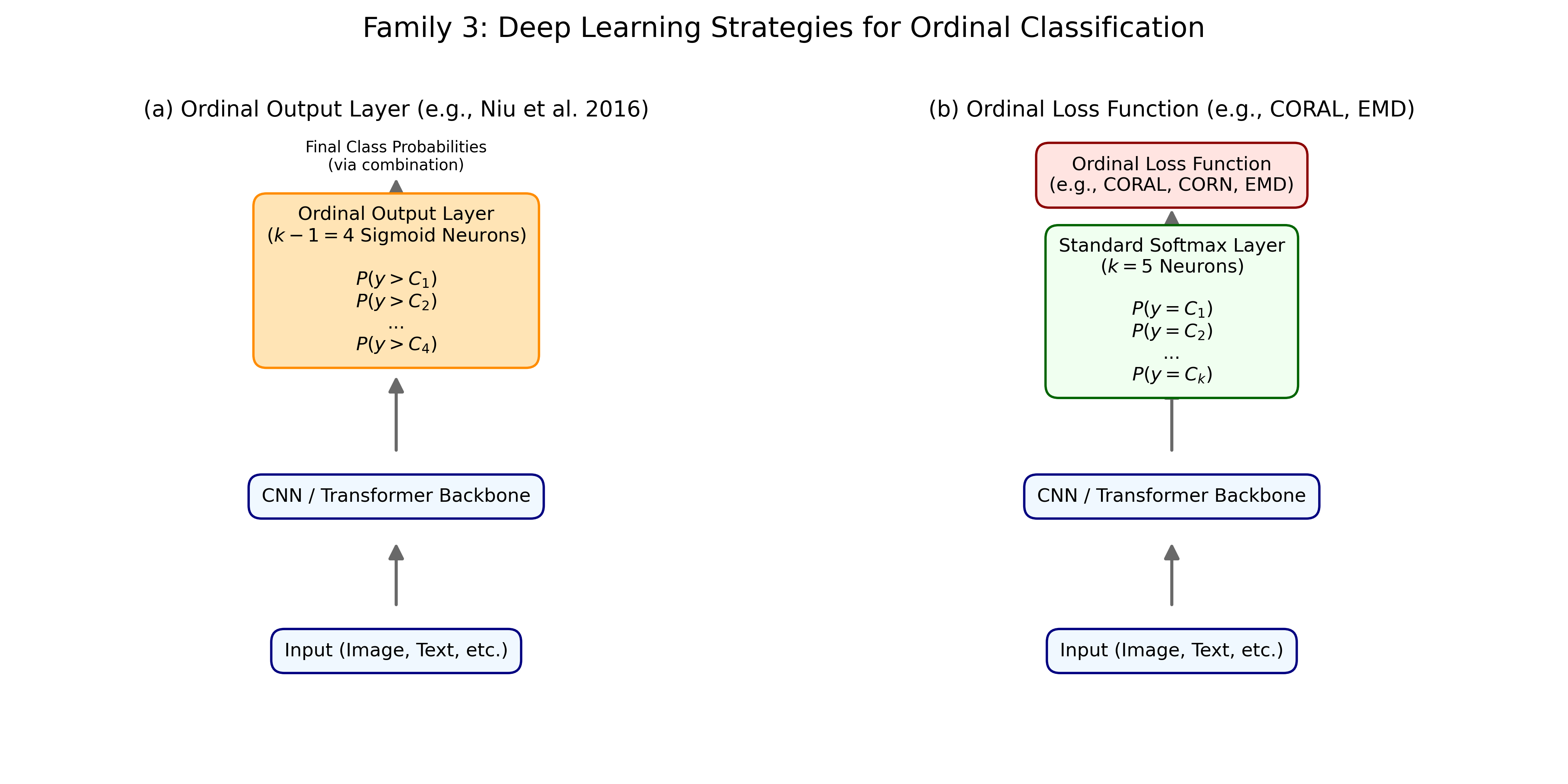
Figure 5.25: Common deep learning strategies for ordinal classification, showing the two approaches tested: (a) The Ordi
Figure 5.25: Common deep learning strategies for ordinal classification, showing the two approaches tested: (a) The Ordi
Ch. 6: Contrastive Learning for Batch
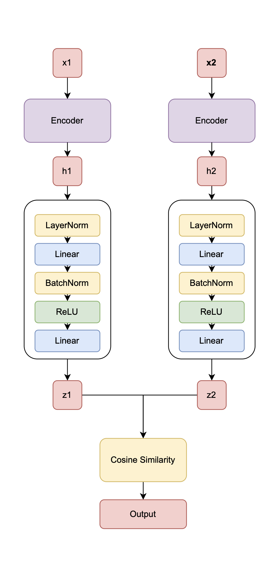
Figure 6.1: SpectroSim Architecture: Paired samples \(x_1\) and \(x_2\) (REIMS spectra) are processed by identical
Figure 6.1: SpectroSim Architecture: Paired samples \(x_1\) and \(x_2\) (REIMS spectra) are processed by identical
Ch. 6: Contrastive Learning for Batch
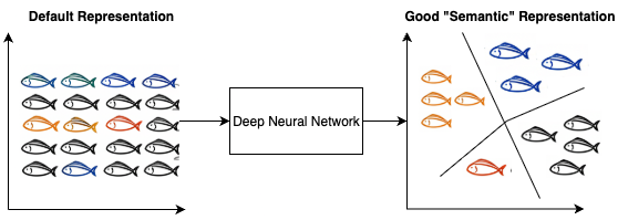
Figure 6.2: This figure illustrates a good ``semantic representation". Imagine that the different colors of fish represe
Figure 6.2: This figure illustrates a good ``semantic representation". Imagine that the different colors of fish represe
Ch. 6: Contrastive Learning for Batch
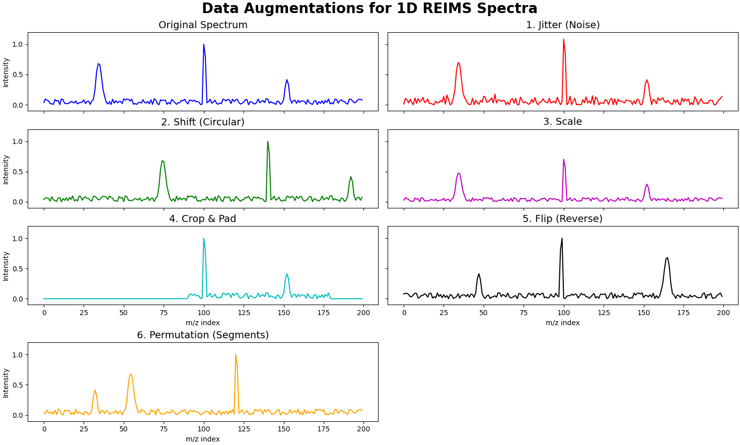
Figure 6.3: Visualization of the six data augmentation techniques described in Section 6.2.2. The Original Spectrum (top
Figure 6.3: Visualization of the six data augmentation techniques described in Section 6.2.2. The Original Spectrum (top
Ch. 6: Contrastive Learning for Batch
Figure 6.4: In the proposed SpectroSim model, we replace the existing ResNet backbone with a Transformer backbone. The c
Figure 6.4: In the proposed SpectroSim model, we replace the existing ResNet backbone with a Transformer backbone. The c
Ch. 6: Contrastive Learning for Batch
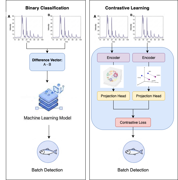
Figure 6.5: This diagram illustrates the difference between binary classification and contrastive learning. Here, we see
Figure 6.5: This diagram illustrates the difference between binary classification and contrastive learning. Here, we see
Ch. 6: Contrastive Learning for Batch
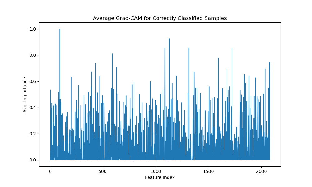
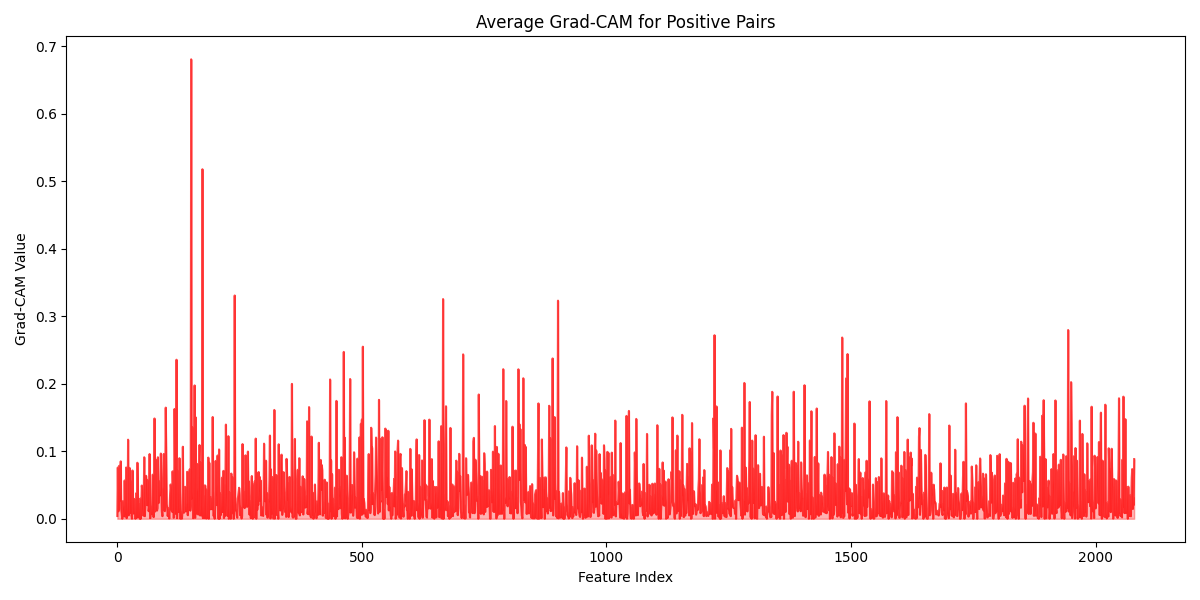
Figure 6.6: Average Grad-CAM for our Transformer-based SpectroSim model. The visualization highlights the most salient m
Figure 6.6: Average Grad-CAM for our Transformer-based SpectroSim model. The visualization highlights the most salient m